How To Make a Line Chart in Excel
Add Trendlines to Excel Charts
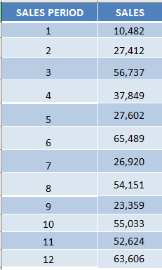
STEP 1: Highlight your table of data, including the column headings:
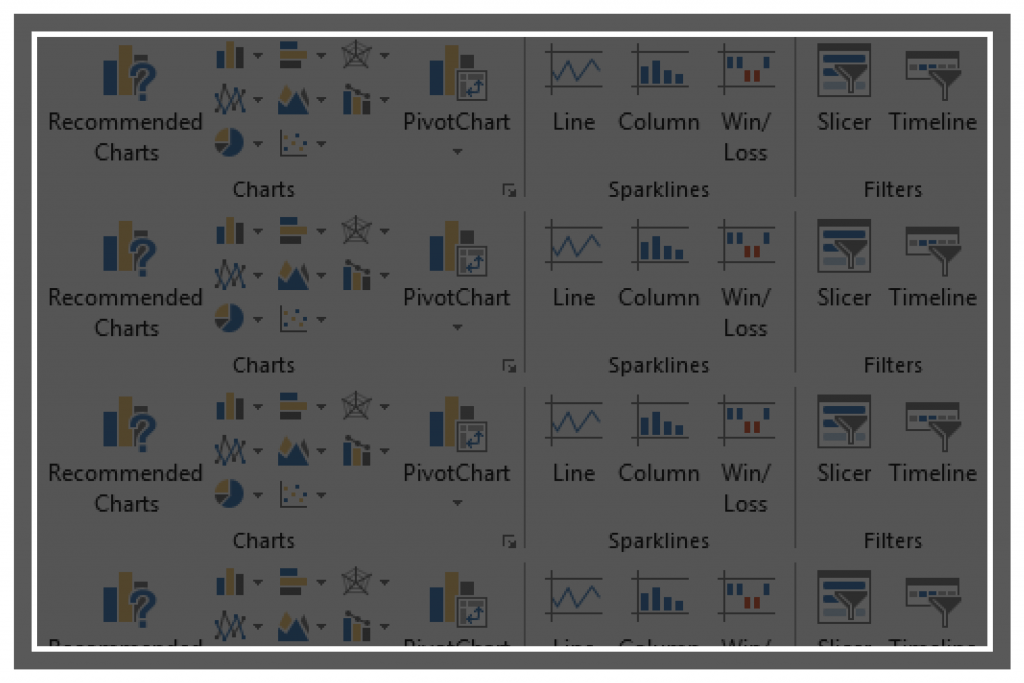
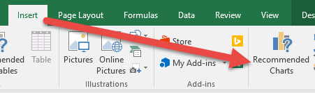
Go to Insert > Recommended Charts (Excel 2013 & 2016)
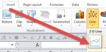
Go to Insert > Line > 2-D Line (Excel 2010)
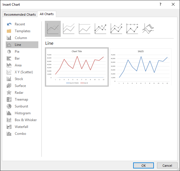
STEP 2: Select All Charts > Line > OK (Excel 2013 & 2016)
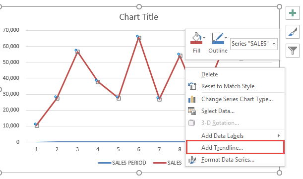
STEP 3: Right click on the line of your Line Chart and Select Add Trendline.
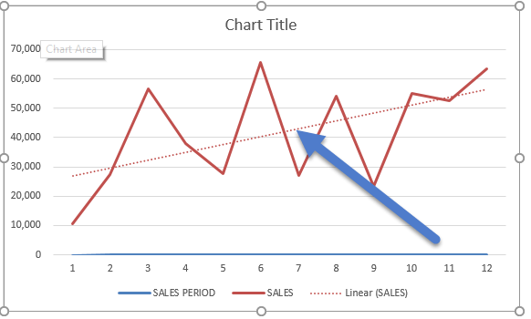
STEP 4: Ensure Linear is selected and close the Format Trendline Window
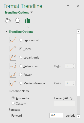
Now you have your Trendline in your chart, and you can predict on where the trajectory is going in the succeeding periods:
Add an Interactive Vertical Column in Your Excel Line Chart
With Excel Charts, it is very easy to create a Vertical Column in your Line Chart and make it interactive with a Scroll Bar!
The reason why I do this, is to use the vertical column to highlight a specific point in my Excel chart whilst I am presenting the data to my stakeholders.
Mmmm Steak :)
In this example, I show you how easy it is to insert an interactive Vertical Column in your chart using Excel & sprinkled with a little magic!
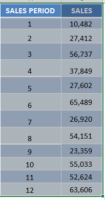
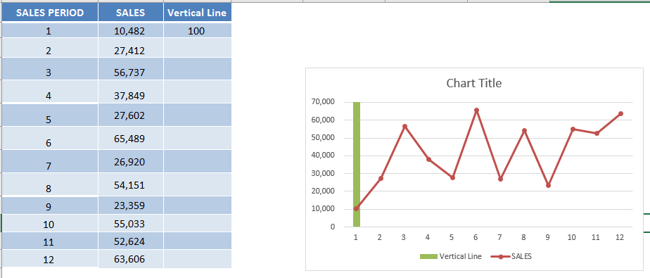
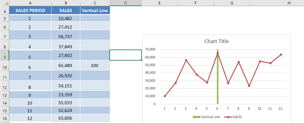
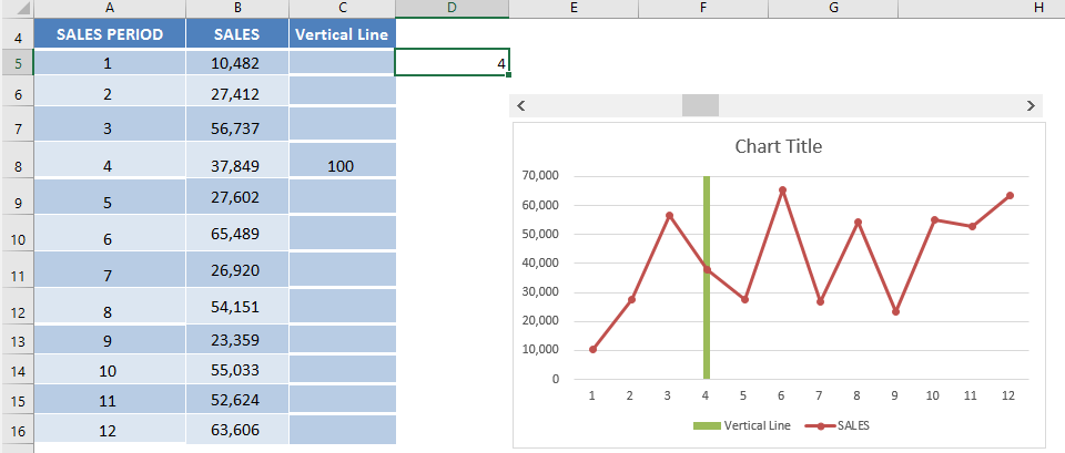
This is our data:
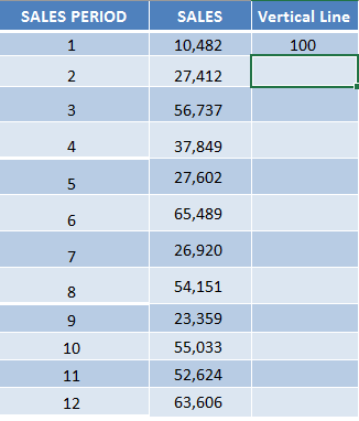
STEP 1: Add a new column Vertical Line, and place in the first value as 100.
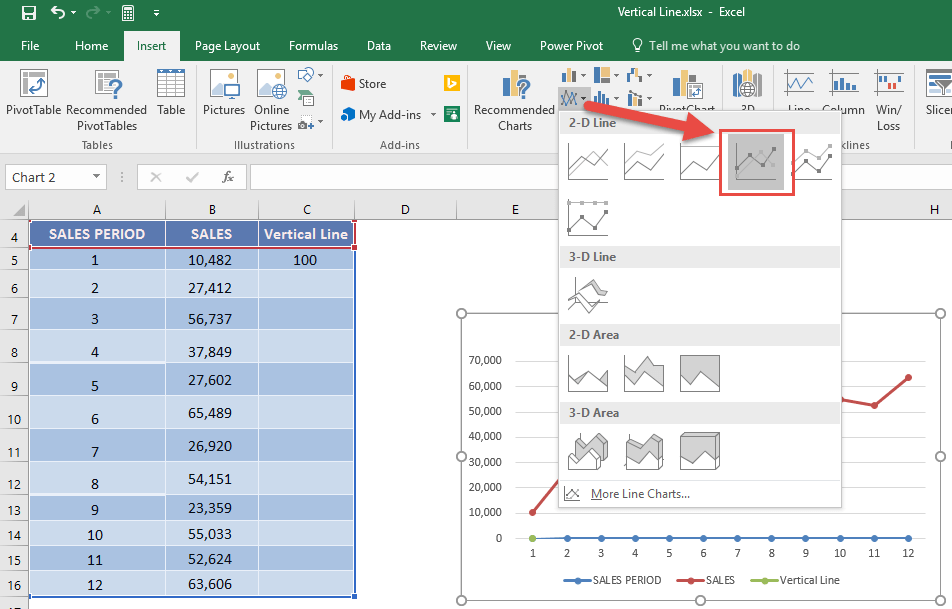
STEP 2: Select the entire table, go to Insert > Line Charts > Line with Markers
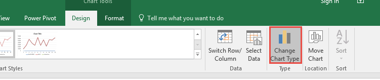
STEP 3: Select the chart and go to Design > Change Chart Type > Combo > Custom Combination
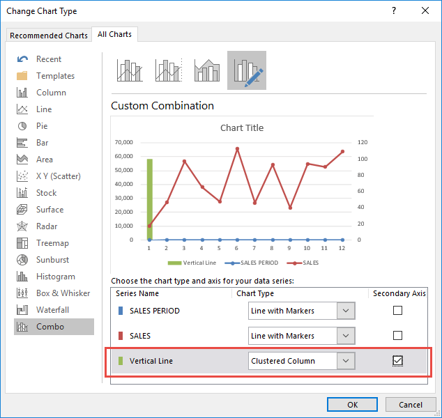
STEP 4: For the Vertical Line series, change the Chart Type to Clustered Column and check Secondary Axis. Press OK.
(This will transform the Vertical Line series into a vertical column in your chart.
Make sure the SALES PERIOD and SALES are Line with Markers Chart Types).
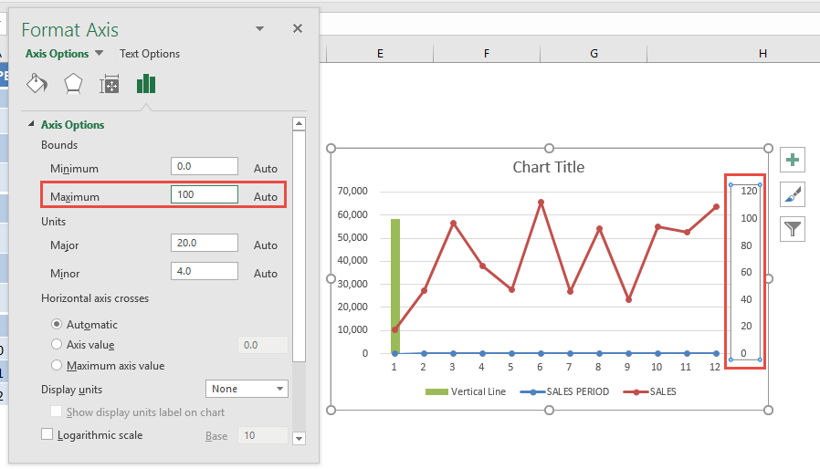
STEP 5: Double click your Secondary Axis to view the Format Axis Panel.
Set Maximum to 100, to ensure our Vertical Line extends all the way to the top since we placed in the value of 100.
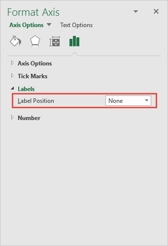
Click on Labels and change the Label Position to None.
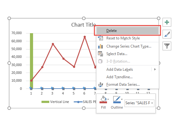
STEP 6: Just to clean up our chart, notice there is a Sales Period Series.
Right click on it and click Delete. We do not need this.
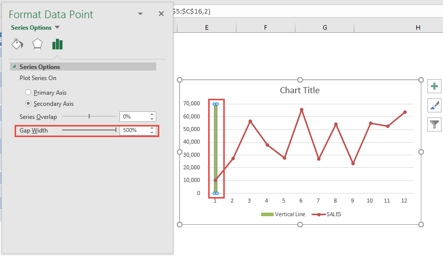
STEP 7: Double click on the vertical bar, so that we can make it slimmer.
In the Format Data Point pane, Set Gap Width to 500%.
STEP 8: Now it is time to try out our interactive chart!
Drag and drop the Vertical Line value of 100 into another Sales Period and see the column chart move!
STEP 9: There is a cooler trick and we can make the Vertical Bar become Dynamic! For this we need the Developer Tab.
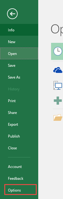
If you do not have Developer Tab enabled yet, it is very easy to enable this first. Go to File > Options
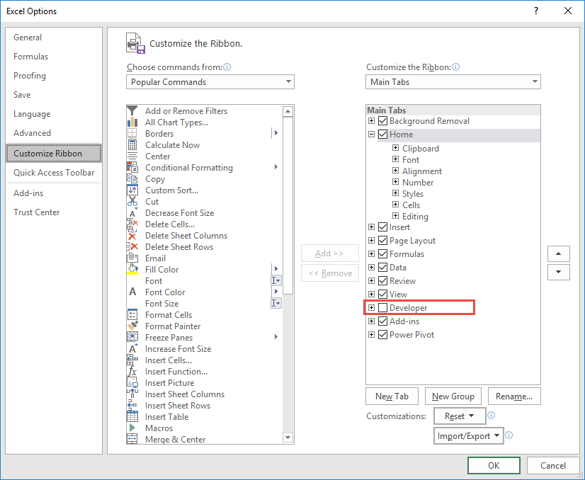
Go to Customize Ribbon > Main Tabs > Developer. Check this and click OK.
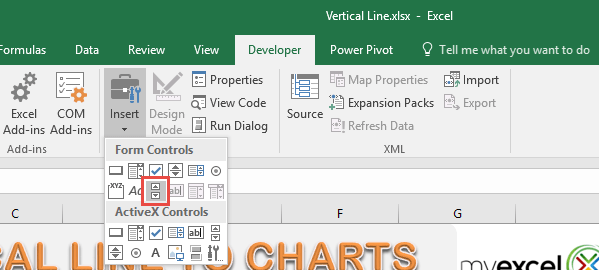
STEP 10: Go to Developer > Insert > Form Controls > Scroll Bar. Drag this horizontally on top of the graph.
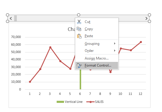
STEP 11: Right click on the scroll bar and select Format Control.
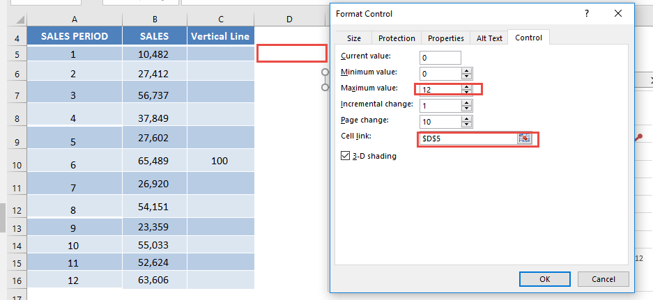
STEP 12: Set the Maximum Value to 12. This will depict our sales periods from 1 to 12.
For the Cell link, place in $D$5, this will show the value of the Scroll bar in this cell (i.e. which sales period it’s pointing to). Press OK.
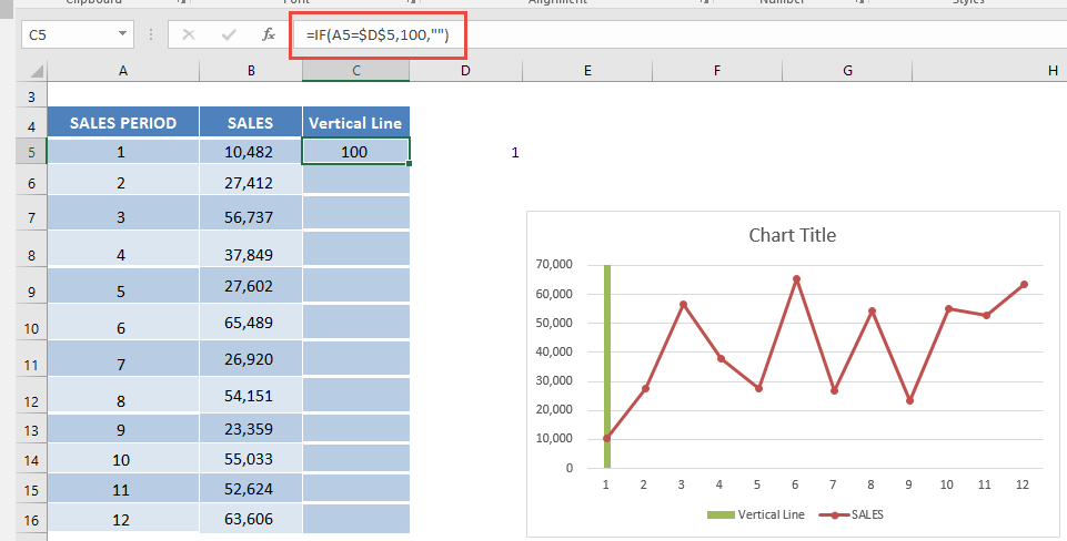
STEP 13: In the Vertical Line column, place in this formula: =IF(A5=$D$5,100,””)
What this will do, is simply check if the Sales Period matches the value of the Scroll bar ($D$5).
If YES, then set the value to 100.
Setting the value to 100, will then make our vertical line show up in that Sales Period!
Now the pieces are almost all in place!
STEP 14: Double click the lower right corner of the formula cell, which will copy the same formula down the entire column.
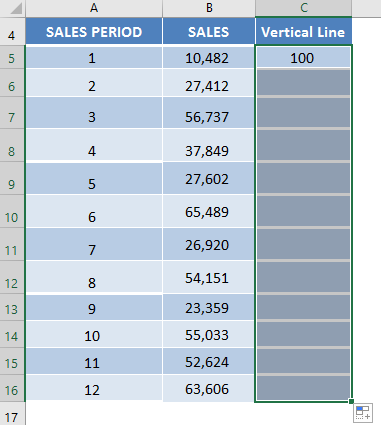
Your interactive chart is now complete!!!
Try playing around with the scroll bar and see the Vertical Line move with it! Cool hey?

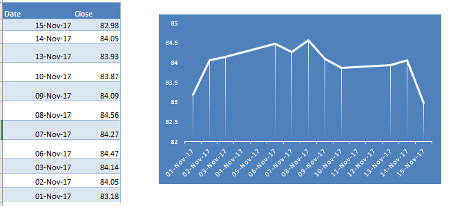
Stock Line Chart Using Excel
Ever had a lot of historical stock data closing prices and you want to visualize how it is going so far?
You can actually use the good old Line Chart in Excel to create your own Stock Line Chart!
Below is the data source that we are going to use to create our Stock Line Chart in Excel:
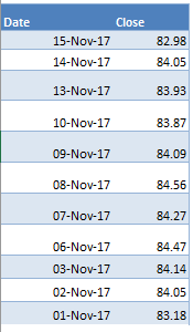
We need 2 data points to create this chart, the Date and the Close Price.
In this example I show you how easy it is to insert a Stock Line Chart using Excel.
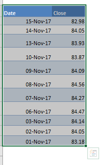
STEP 1: Highlight your data of stock prices:
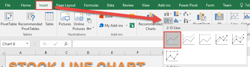
STEP 2: Go to Insert > Line Charts > Line
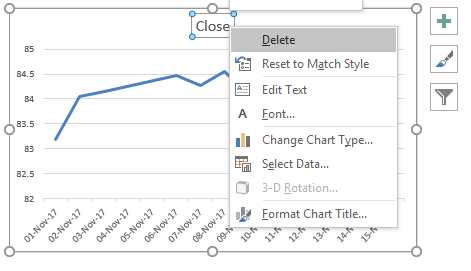
STEP 3: Right click on your Title and choose Delete as we do not need this.
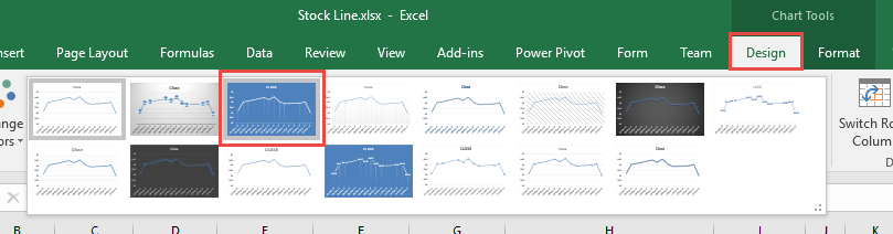
STEP 4: Go to Chart Tools > Design and select the preferred design to make your chart more presentable!
And there you have it! Your own Stock Line Chart in Excel!