Enabling Power Pivot Excel 2016

Power Pivot is an Excel add-in that was first introduced in Excel 2010 by Microsoft. It allows you to harness the power of Business Intelligence right in Excel.

Read the tutorial on how to install Power Pivot in Excel 2010 here

Read the tutorial on how to enable Power Pivot in Excel 2016 here

In this tutorial, you will be provided with a detailed guide on

• What is Power Pivot?
• How to Enable Power Pivot for Excel 2016?
• Getting started with Power Pivot 2016
  • How to open the Power Pivot window?
  • Add Data to Data Model
  • Different Views in Power Pivot
  • Create Relationship in Power Pivot
  • Create Pivot Table using Power Pivot data
• Advantages of using Power Pivot Excel 2016
• Conclusion

Let’s go through each point one-by-one!

 

What is Power Pivot?

Power Pivot gives you the power to work with large sets of data.

In a nutshell, it allows you to use multiple data sources. Then you could import, merge and perform analysis on the resulting data.

The beautiful thing with Power Pivot is it allows you to work on Big Data with no limitations.

Imagine getting data from multiple sources like SQL Server, Oracle, XML, Excel, Microsoft Access then build a Data Model from it. Then you can analyze these all into one awesome Pivot Table!

 

How to Enable Power Pivot for Excel 2016?

So how do I get my hands on this super awesome add-in…I hear you say?

The good thing with Power Pivot is it already comes with your Excel 2016, we need to enable it to start using Power Pivot.

You just need to make sure you have one of these versions:

Office 365 Pro Plus

Office 365 E3

Power Pivot is NOT AVAILABLE in Office 2016 for the following products:

Office 365 Home, Office 365 Personal, Office 365 Business Essentials, Office 365 Business, Office 365 Business Premium, Office 365 Enterprise E1

 

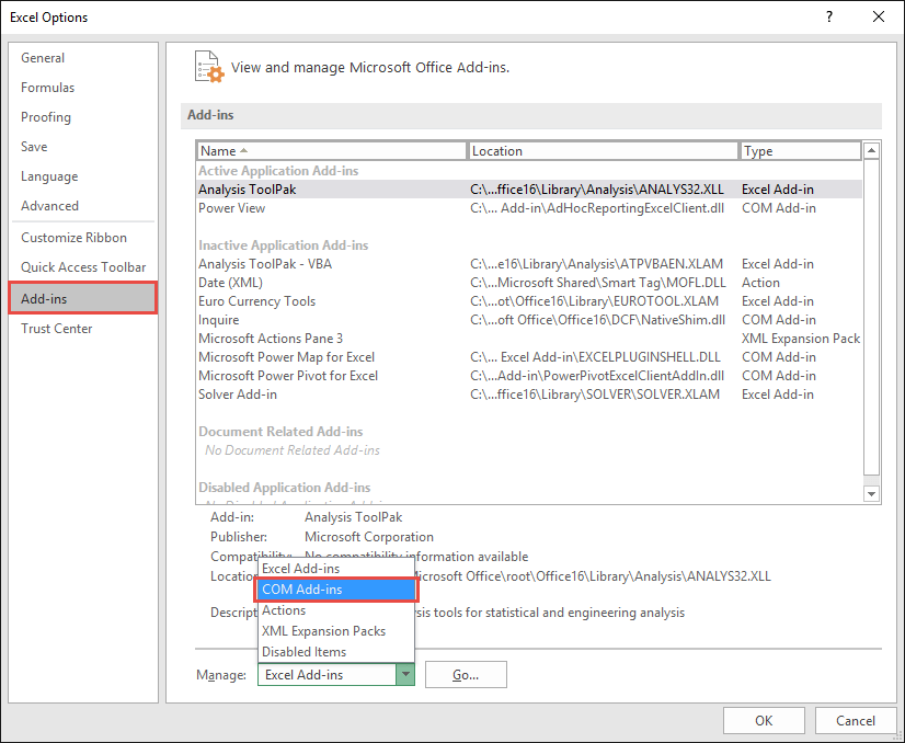
STEP 1: Go to File > Options 

 

STEP 2: Go to Add-Ins, for the Manage dropdown select COM Add-ins. Click Go once set.

 

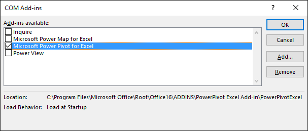
STEP 3: Check Microsoft Power Pivot for Excel. Click OK once done.

You can easily enable Pivot Excel 2016 download and make the tab appear in the menu ribbon.

STEP 4: You should now have the Power Pivot Tab.  Click Manage to see the Power Pivot Window.

This will open Power Pivot in Excel 2016!

 

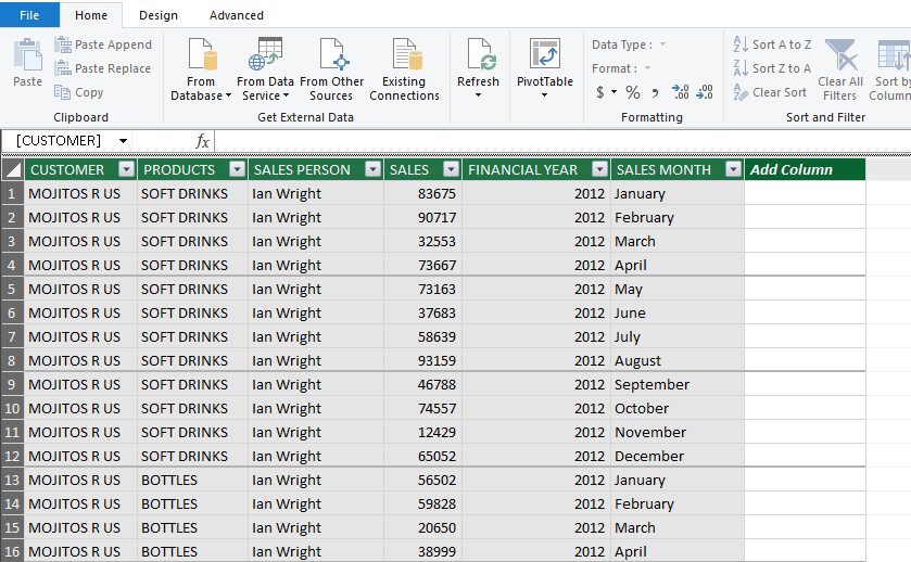
Power Pivot Window (click on the image to expand):

 

Getting Started with Power Pivot Excel 2016

To work on Power Pivot, you must first understand how to open the Power Pivot window.

 

How to open the Power Pivot window?

STEP 1: Click on the Power Pivot Tab in Menu Ribbon.

STEP 2: Select the Manage option under Data Model.

This opens the Power Pivot window and here you can explore all of its features!

 

Adding Data to Data Model

The first step is to add some data to your model. You can import data from two categories:

• From the Current Workbook
• From External Data Sources.

Let’s talk about each one of them in detail.

 

To Import data from the Current Workbook, follow the steps below:

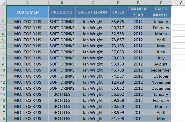
STEP 1: Highlight the Data in your current workbook.

 

STEP 2: Go to Insert > Table to convert data into a table.

 

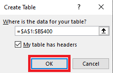
STEP 3: In the Create Table dialog box, Click OK.

 

STEP 4: Go to Power Pivot > Add to Data Model.

This will import the data into the power pivot window.

 

To Import data from an External Data Source like an Excel File, follow the step-by-step tutorial below:

STEP 1: Click on Power Pivot > Manage to open the Power Pivot Window.

STEP 2: Click on Home > From Other Sources.

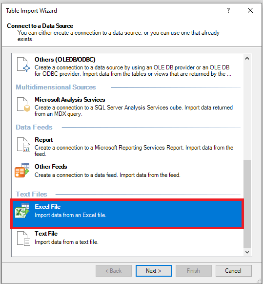
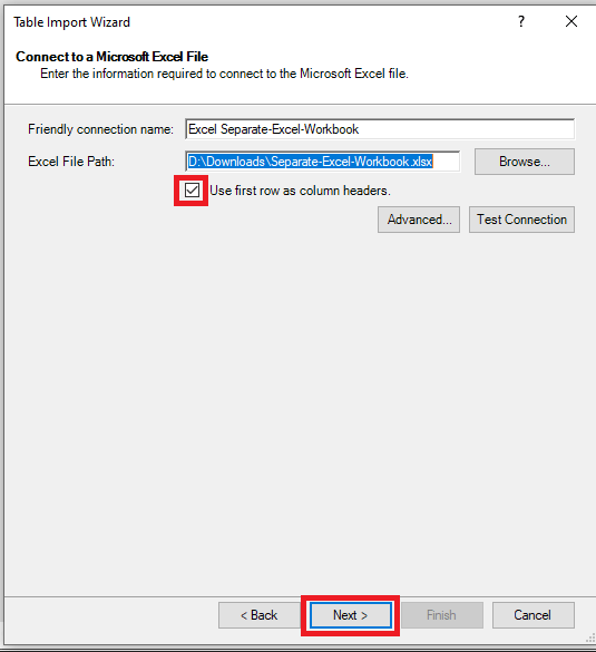
STEP 3: In the Table Import Wizard, Select Excel File and Click Next.

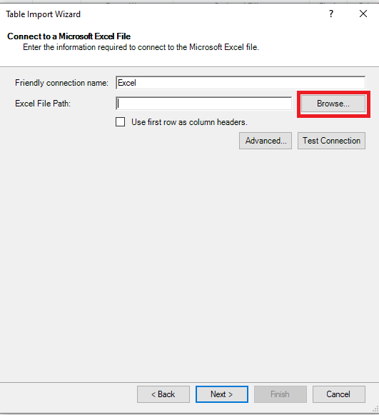
STEP 4: Click on Browse. 

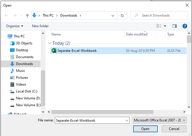
STEP 5: Select the Excel file that you want to import.

STEP 6: Click Next. Make sure to check the box for Use first row as column headers.

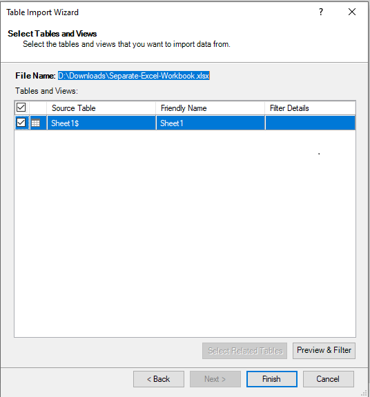
STEP 7: Click Next (As the desired sheet is already selected here)

If you have multiple sheets in your file, it will be displayed here and you can select the one you want to import.

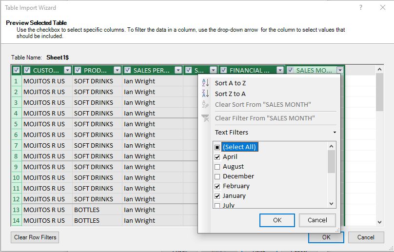
If you also apply a filter in your data as per your required. Say, you want to display data for the month of  January, February, and April only.

You can do that by clicking on the Preview & Filter button and then applying the filter.

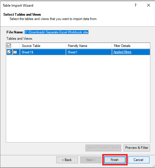
Only the filtered data will be imported to Power Pivot.

STEP 8: Click Finish.

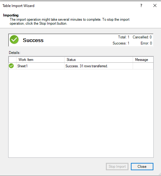
STEP 9: A Success message will be displayed showing you the number of rows that have been imported. Verify that and Click Close.

 

Different Views in Power Pivot

There are two views that are available in Power Pivot – Data View and Diagram View.

Data View

This is the view shown to Excel users by default.

Data view displays a table of your data model in a grid format, much like the standard Excel. Each table has its own tab at the bottom of the sheet. You cannot make any edits in the cells in the data view.

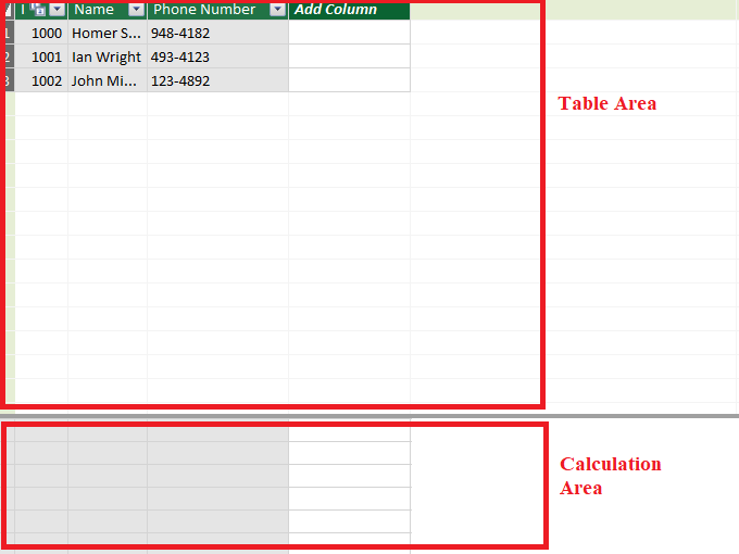
A data view is comprised of two parts – the Table area and the Calculation area.

The Table area is where the data table is displayed and the Calculation area is just below the table area where you can create measures.

You can even hide the Calculation area if it is not required by clicking on the Home > Calculation Area.

Diagram View

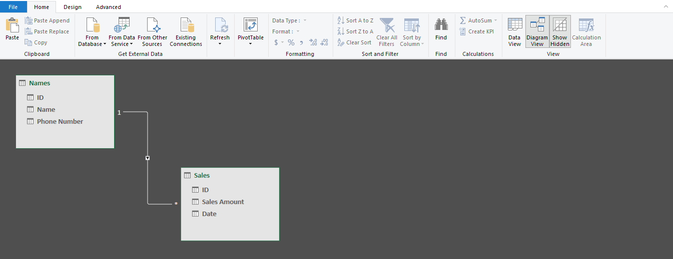
Ever faced a situation when you have multiple tables in Power Pivot and you are unable to analyze the relationship?

Diagram View provides a perfect solution for this problem – a bird’s eye view for all your tables.

Let’s look at an example of how data is displayed in Diagram View.

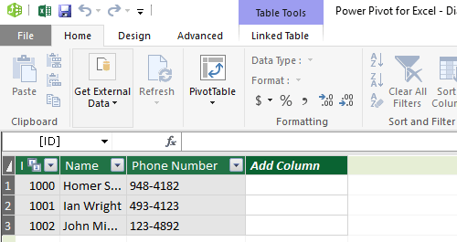
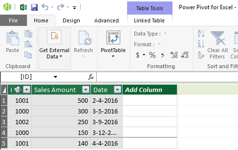
You have two tables – Names and Sales.

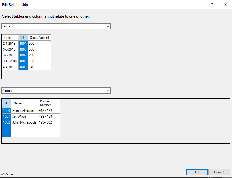
Names Table

Sales Table

The ID column of the Sales Table is linked to the ID column of the Name Table.

*** You can view the exact step-by-step tutorial of how this was done here: Linking Excel Tables in Power Pivot. ***

To get a bird’s eye view of this relationship, Go to Home > Diagram View

In Diagram View, each table is represented using a box with the header as table name, and then below is the name of the columns of that particular table.

You can drag the corner of the table to resize them and can also move them to different locations.

 

Create Relationship in Power Pivot

In the example above, you have imported the two tables in the Power Pivot window. You can now link the ID column from the Names table with the ID column in Sales Table.

Let’s see how it can be done by following the steps below:

STEP 1: In the Power Pivot window, Go to Home > Diagram View.

STEP 2: Select the Column Heading and drag to connect it to the Column heading of the second table.

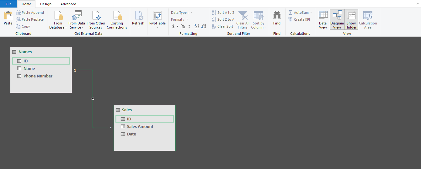
To view the relationship created, simply double click on the arrow linking the two tables.

As you can see the ID column is highlighted in both the tables indicating the link between the two columns.

 

Create Pivot Table using Power Pivot data

STEP 1: Click on the Power Pivot Tab in Menu Ribbon.

STEP 2: Select the Manage option under Data Model.

STEP 3: In the Power Pivot window, Go to Home > PivotTable.

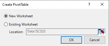
STEP 4: In the Create PowerTable dialog box, Select New Worksheet and click OK.

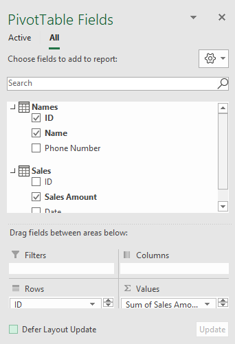
STEP 5: In the PivotTable Fields panel, you can drag and drop fields to create a customized PivotTable.

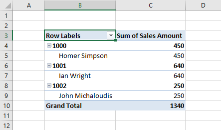
This is how the PivotTable will look like:

 

Advantages of using Power Pivot Excel 2016

The main advantages of using Power Pivot Excel 2016 are as follows:

• You can work with millions of rows and extract data from multiple sources.
• You can process calculations and analysis faster.
• You can import data from multiple sources and you can also filter data and rename columns while importing.
• When you import a table in Power Pivot, each table gets organized in individual tabbed pages.
• You can create your own formula using DAX expression.
• You can create relationships among the table to easily analyze data fields together.
• You can create calculated fields and calculated columns in the data table.

 

Conclusion

In this article, you have learned about Power Pivot Excel 2016 download- how to install Power Pivot for Excel 2016, Open a power pivot window, add data to model from current file or external sources, different views in power pivot excel 2016, and lastly the advantages of using Power Pivot.

There is a lot you can do using this tool. Click here to learn more.

Further Learning:

• Importing Excel Workbooks in Power Pivot
• Using the Diagram View in Power Pivot
• Unpivot Data Using Excel Power Query

You can learn more about how to use Excel by viewing our FREE Excel webinar training on Formulas, Pivot Tables, and Macros & VBA!

>