How to Calculate Returns with Excel MIRR Function

Ever wanted a tool to delve deeper into investment profitability? Enter Microsoft Excel‘s Modified Internal Rate of Return (MIRR) function, a game-changer in the world of financial analysis. Unlike traditional metrics, MIRR factors in costs and reinvestment rates, offering a clearer view of project or investment viability. With MIRR, steer clear of misleading figures and unlock the true potential of your investment decisions.

Key Takeaways:

• Seamless Analysis: MIRR in Excel simplifies Return on Investment (ROI) analysis, minimizing complexity and errors, so you can focus on strategic decisions.
• Setup Made Easy: Understand MIRR’s inputs—initial investment, cash flows, finance rate, and reinvestment rate—to lay a solid foundation for accurate analysis.
• Interpretation Insights: Higher MIRR indicates more profitable investments, while lower values might signal underperformance, guiding your investment choices.
• Comprehensive Evaluation: Use MIRR alongside other metrics for a holistic view of investments, ensuring informed decision-making.
• MIRR vs IRR: While both are valuable, MIRR’s consideration of reinvestment rates offers a more conservative and precise analysis compared to IRR.

 

Unlocking the Potential of MIRR in Excel

Deciphering MIRR for Smarter Investment Decisions

Imagine a tool that could offer you a deeper insight into the profitability of your investments, allowing for smarter decision-making. That’s precisely what the Modified Internal Rate of Return (MIRR) function in Excel does. Unlike traditional metrics, MIRR incorporates the financial reality of costs and reinvestment rates, enabling a more robust analysis of your projects or investments. With MIRR, you’ll discover the true potential of your investment decisions, steering clear of misleading figures that could hurt your financial future.

With the right know-how, Excel’s MIRR function can become your trusty partner in navigating the intricate world of investment returns. It helps you take into account various investment cash flows over time, providing a more accurate picture of an investment’s profitability by considering both the cost of investment and the reinvestment of returns. In essence, MIRR adjusts for the time value of money, allowing you to compare different investments with varying cash flows seamlessly.

A Calculator that Makes ROI Analysis Painless

You know how complex and overwhelming the Return on Investment (ROI) analysis can be. But guess what? It doesn’t have to be. Think of the MIRR function in Excel as your personal calculator that streamlines the process, making the ROI analysis virtually painless. Just key in your initial investment, periodic cash flows, finance rate, and reinvestment rate; Excel will handle the intricate math.

This eliminates the need for tedious manual calculations and reduces the chance of errors, so you can focus on interpreting the results for a savvy investment strategy.

 

Set Up Your Quick & Easy MIRR Calculator

Laying the Groundwork: Understanding MIRR’s Inputs

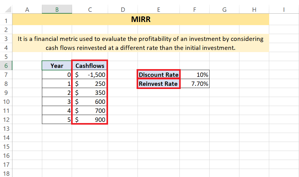
Before diving into the actual computation, it’s crucial to understand the nuts and bolts of what goes into a MIRR calculation. The inputs you’ll need are the initial investment, the series of periodic cash flows, the finance rate, and the reinvestment rate.

The initial investment usually takes a negative value, representing the cash outflow, while the series of cash flows can be a mix of negative and positive figures over time, reflecting the net movements of money. The finance rate is the cost of capital or the interest rate paid on the money used for the investment. On the flip side, the reinvestment rate is the rate of return expected on the re-investment of the cash flows.

Understanding each component helps you grasp the complete picture of what your MIRR result will imply. Each input plays a significant role in the overall calculation, offering a precise measure of an investment’s attractiveness. Consider these inputs as the solid foundation upon which your financial analysis will be built. Getting them right is some sort of an art — and certainly a science you can master!

Punching the Numbers: Step-by-Step MIRR Setup

When you’re ready to get your hands on Excel’s MIRR function, the setup is straightforward. Here are the simple steps to follow, ensuring you punch in the numbers correctly:

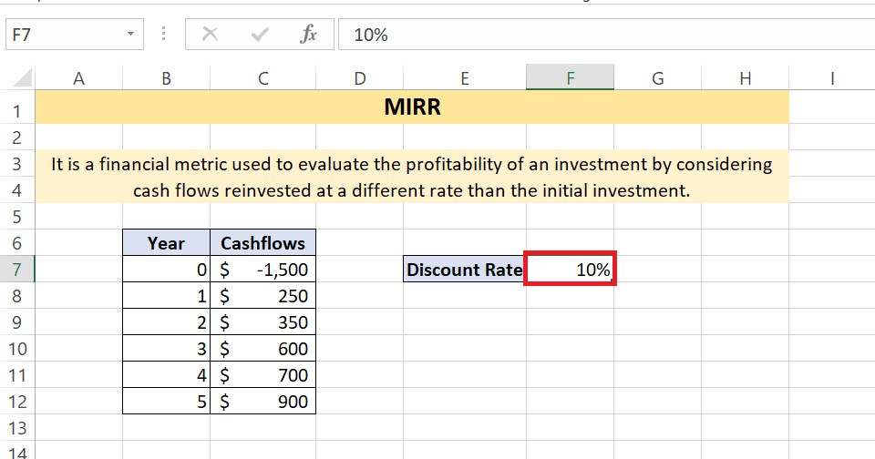
STEP 1: Collect all necessary data, including your series of cash flows, the initial investment amount, the finance rate, and the reinvestment rate.

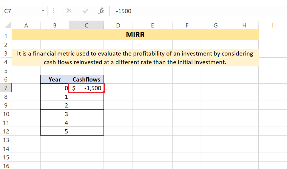
STEP 2: Open Excel and input your initial investment (as a negative number) into one cell.

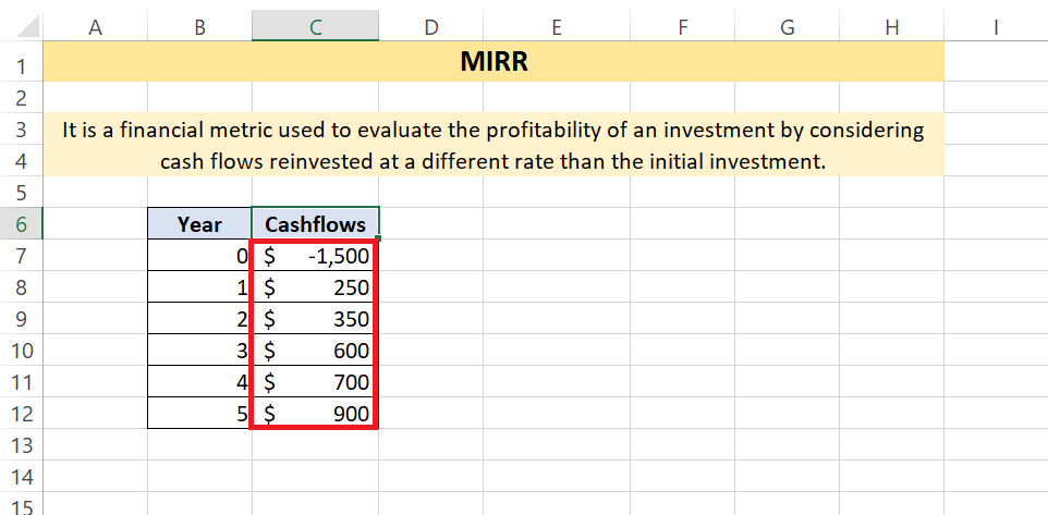
STEP 3: In adjacent cells, enter your periodic cash flows, which can be positive or negative, corresponding to the money coming in or going out.

STEP 4: Designate a cell for the finance rate, which represents your cost of borrowing or investing capital.

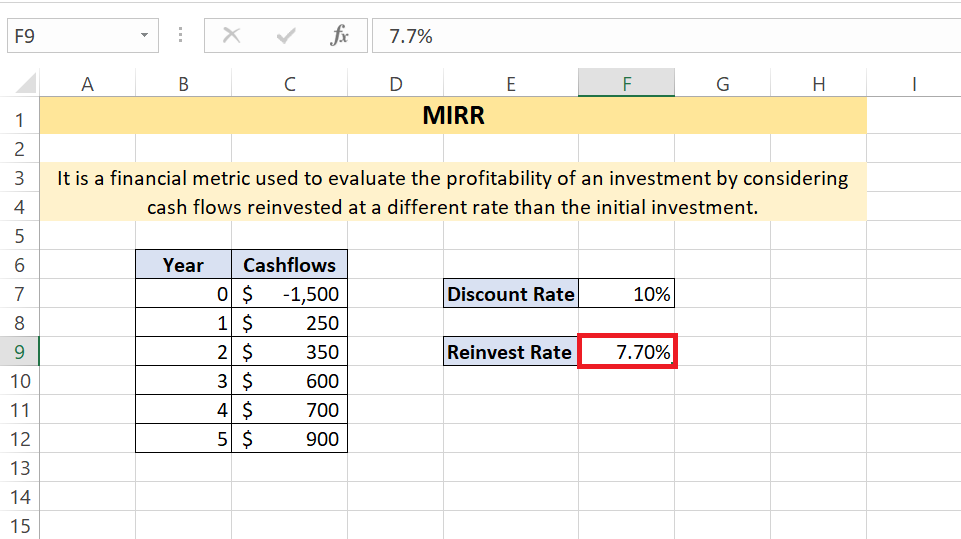
STEP 5: Specify another cell for the reinvestment rate, the rate you assume the investments’ cash flows will earn.

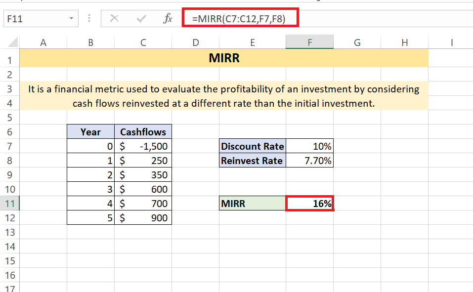
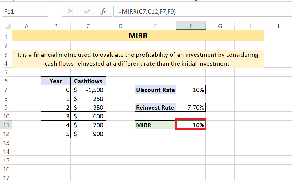
STEP 6: Click on the cell where you wish to see your MIRR result, type “=MIRR(“, and then select the range of cash flows, include the finance rate, and the reinvestment rate cells. Finish by typing “)” i.e, “=MIRR(C7:C12,F7,F9)” and hit Enter.

And voilà! Excel does the heavy lifting, and your MIRR result pops up, ready to inform your investment analysis. Remember, this quick setup not only saves you time but also provides a high degree of accuracy.

 

Analyzing Results for Better Financial Insight

Interpreting MIRR Outcomes for Clearer Investment Choices

The moment of truth arrives as you interpret the MIRR outcomes, which now lay the path to clearer and more strategic investment choices. A higher MIRR signifies a more desirable investment, suggesting that the project’s returns more than compensate for your cost and reinvestment expectations. Conversely, a lower MIRR can be a red flag, indicating potential underperformance or that the investment might not meet your financial targets.

Don’t just glance and go! Dive deep into what these percentages represent — are they aligned with your risk tolerance? Do they surpass benchmark returns? MIRR speaks volumes about long-term growth potential, and your next move might just be driven by the insights that this powerful function provides.

Keep in mind that while MIRR is a robust tool, it should be part of a wider financial analysis, complementing other factors and metrics to paint the full investment picture. Trust MIRR to provide a trustworthy estimate that factors in essential financial variables, but remember that due diligence never stops at just one metric.

Case Study- Comparing Investments with Varying MIRR Outcomes Scenario:

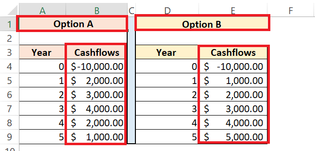
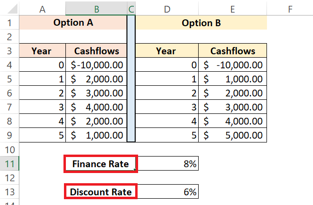
Suppose you have $10,000 to invest and are considering two investment options: Option A and Option B. Both options have different cash flows over a five-year period.

STEP 1: Calculating MIRR:

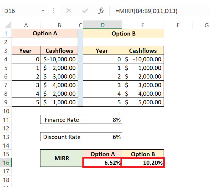
Using Excel, apply the MIRR formula for both options, considering a finance rate of 8% and a reinvestment rate of 6%.

STEP 2: Interpretation:

·Option A: MIRR = 6.52%

·Option B: MIRR = 10.20%

Comparison: Option B has a higher MIRR, indicating potentially greater profitability after considering both the initial investment and reinvested cash flows.

Decision: If maximizing returns is the primary goal, Option B appears more favorable due to its higher MIRR, suggesting better utilization of reinvested cash flows.

Conclusion: In investment decision-making, considering MIRR alongside other financial metrics provides a comprehensive understanding of the potential profitability of different options. In this case, Option B demonstrates higher potential returns, emphasizing the importance of evaluating investments beyond their initial costs.

 

FAQ: All Your MIRR Questions Answered

How to calculate MIRR with Excel?

To calculate MIRR in Excel, enter all cash flows, including the initial investment as a negative number, in a column. Then, in a separate cell, enter the formula =MIRR(range of your cash flows, finance rate, reinvestment rate), replacing the placeholders with the appropriate cell ranges and rates. Press Enter, and Excel will display the MIRR. Make sure your finance and reinvestment rates are expressed as decimals (e.g., 5% as 0.05).

What Exactly Does the MIRR Function Do in Excel?

The MIRR function in Excel calculates the Modified Internal Rate of Return for a series of periodic cash flows. It adjusts for the timing of cash flows, considering both the cost of investment (finance rate) and the profit from reinvesting cash flows (reinvestment rate), to give a more accurate measure of an investment’s profitability.

Can MIRR Serve as a Standalone Tool for Financial Analysis?

While MIRR is a powerful tool for evaluating the viability of investments, it’s best used in conjunction with other financial measures. Alone, it can’t capture all aspects of investment risks or opportunities. A comprehensive analysis would typically include MIRR among a suite of other metrics for thorough decision-making.

Does the MIRR Include Reinvestment Rate in Calculations?

Yes, MIRR includes the reinvestment rate in calculations. It’s a critical input that reflects the rate of return for reinvesting the cash flows from the investment, providing a comprehensive view of the investment’s potential profitability.

What is MIRR vs IRR in Excel?

In Excel, MIRR accounts for both the cost of investment and the rate of reinvestment, offering a more realistic picture of an investment’s yield compared to IRR, which only assumes reinvestment at the project’s own rate of return. Both are valuable, but MIRR often provides a more conservative and precise analysis.