How to Calculate Hours and Minutes Worked in Excel Fast

Microsoft Excel is a powerful tool designed to simplify time calculations, from simple time tracking to complex scheduling scenarios. When you’re dealing with hours and minutes for payroll or project management, understanding how to efficiently calculate time in Excel can save you countless hours and reduce errors. In this blog post, we will dive into the essential techniques and formulas necessary to calculate hours and minutes worked in Excel.

Key Takeaways:

• Correct formatting is crucial: Always use consistent time formats like 24-hour (hh:mm) to avoid confusion in calculations.
• Basic time subtraction works well: Subtracting the start time from the end time using =EndTime – StartTime gives accurate hours worked.
• Account for break times: Use =(EndTime – StartTime) – BreakTime to deduct unpaid breaks for precise results.
• Use custom formats for clarity: Applying [h]:mm ensures that Excel displays time sums correctly, even beyond 24 hours.
• The TEXT function improves display: Use =TEXT(…, “h:mm”) to format elapsed time neatly for reports and presentations.

 

Getting Started with Time Calculations

Setting Up Your Data for Success

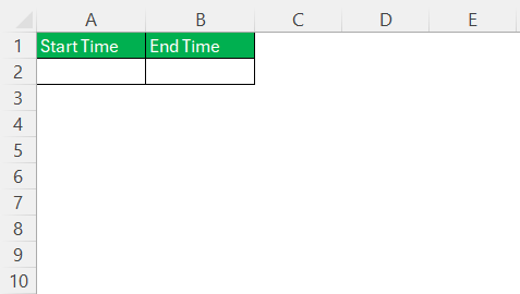
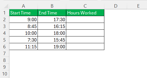
Before delving into calculations, it’s crucial to ensure your data is set up correctly. Begin by entering your start and end times in separate columns. For best results, use the 24-hour format (e.g., 14:00 instead of 2:00 PM) to avoid confusion with AM/PM designations.

Label your columns clearly, such as “Start Time” and “End Time,” to facilitate simple and error-free calculations.

This foundational setup will lay the groundwork for your time calculations and help maintain data consistency.

Understanding Time Formats in Excel

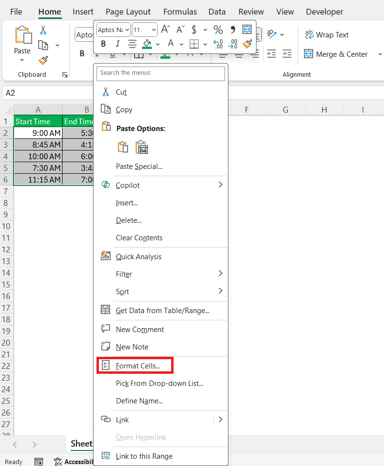
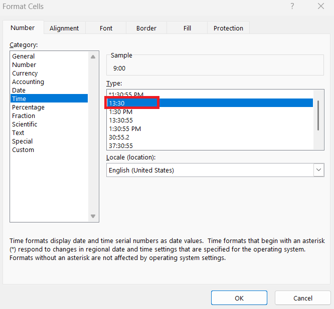
Excel offers various time formats to suit different needs, with the most common being ‘hh:mm’ and ‘hh:mm:ss.’ This formatting plays a pivotal role because it dictates how Excel interprets and calculates time values. The ‘hh:mm’ format is suitable for hours and minutes, while ‘hh:mm:ss’ includes seconds for more detailed logging. To apply these formats, select your cells and right-click to open the format menu.

Choose ‘Format Cells,’ then under the ‘Number’ tab, select ‘Time’ and pick the desired format.

Understanding these formats is essential to ensure your formulas yield accurate results.

 

Calculate Hours and Minutes Worked

How to Use Simple Time Difference Formulas

Calculating the difference between start and end times in Excel is a fundamental operation that can be executed with simple formulas. Here’s how you can do it efficiently:

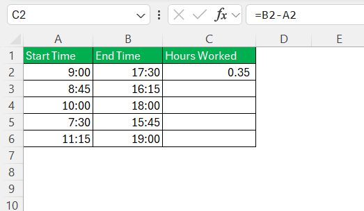
STEP 1: In a new column, label it “Hours Worked” to keep your calculations organized.

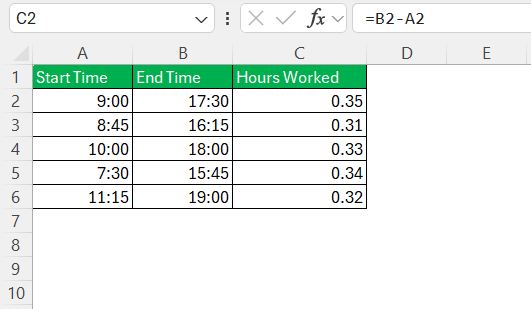
STEP 2: In the first cell under the “Hours Worked” column, enter the formula =End Time Cell - Start Time Cell (e.g., =B2-A2), where B2 contains the end time and A2 contains the start time.

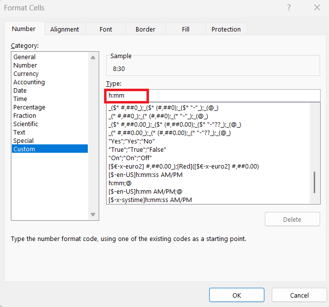
STEP 3: Format the result cell as ‘h:mm’ to ensure the outcome appears as hours and minutes worked.

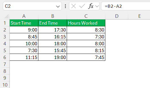
STEP 4: Click and drag the fill handle to copy the formula down the column to apply it to other rows, efficiently calculating the difference for each entry.

Using this simple time difference formula allows you to quickly compute hours worked across a variety of scenarios, facilitating time management and payroll calculations with ease.

Subtracting Breaks and Unpaid Time

To account for breaks and unpaid time in your work hour calculations, you can enhance your existing formula. Here’s how:

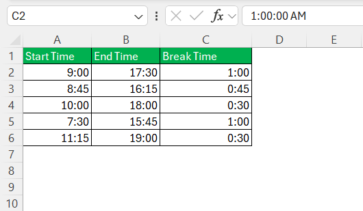
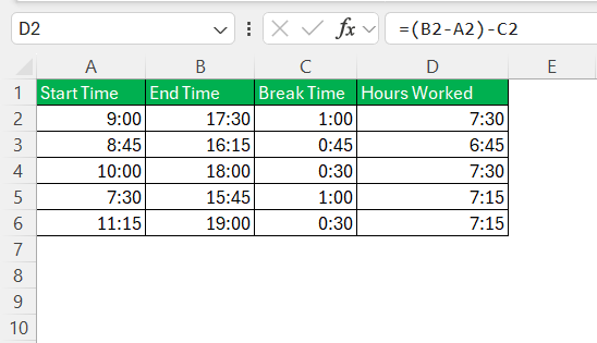
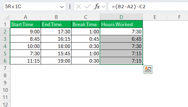
STEP 1: Add a new column named “Break Time” to list the duration of breaks taken during the work period. Input these values in ‘hh:mm’ format for consistency.

STEP 2: In the “Hours Worked” column, adjust your existing formula to subtract break times. For instance, use =(End Time - Start Time) - Break Time (e.g., =(B2-A2)-C2), where C2 contains the break duration.

Again, drag the formula down the column to apply it to all relevant rows.

By systematically subtracting breaks and unpaid time, you can derive a more precise calculation of hours worked, aiding in fair compensation and transparent time tracking.

 

Advanced Tips & Tricks

Using the TEXT Function for Elapsed Time

The TEXT function in Excel is versatile and can be used to display elapsed time in a specific format, enhancing readability and presentation. Here’s a guide to using the TEXT function for this purpose:

STEP 1: Initially, use a basic formula to find the time difference, such as =End Time - Start Time.

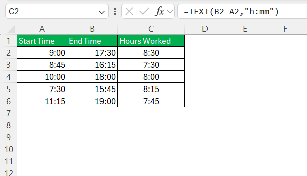
STEP 2: To format the elapsed time, wrap the basic formula with the TEXT function. For example, use =TEXT(End Time - Start Time, "h:mm"). This ensures the time is displayed as ‘hours:minutes’.

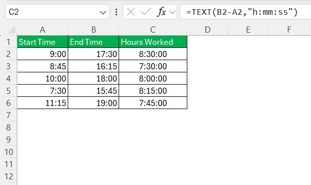
STEP 3: If you need a more detailed format, including seconds, modify the formula to =TEXT(End Time - Start Time, "h:mm:ss").

This formatted result is particularly useful in reports where a consistent presentation improves clarity. The TEXT function doesn’t handle negative times gracefully. Ensure your time calculations don’t inadvertently lead to negative results with overnight shifts.

Using the TEXT function can help make your data more accessible and visually consistent, especially in documents that will be shared with others or used for presentations.

Summing Over 24 Hours Easily

Summing time values that exceed 24 hours in Excel requires special handling to display the result correctly as cumulative hours. Here is a step-by-step approach to do it efficiently:

STEP 1: Highlight the cells containing the time values that need to be added together.

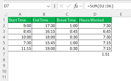
STEP 2: In the cell where you want the total displayed, input the formula =SUM(Cell Range), replacing ‘Cell Range’ with your actual range (e.g., =SUM(D2:D6)).

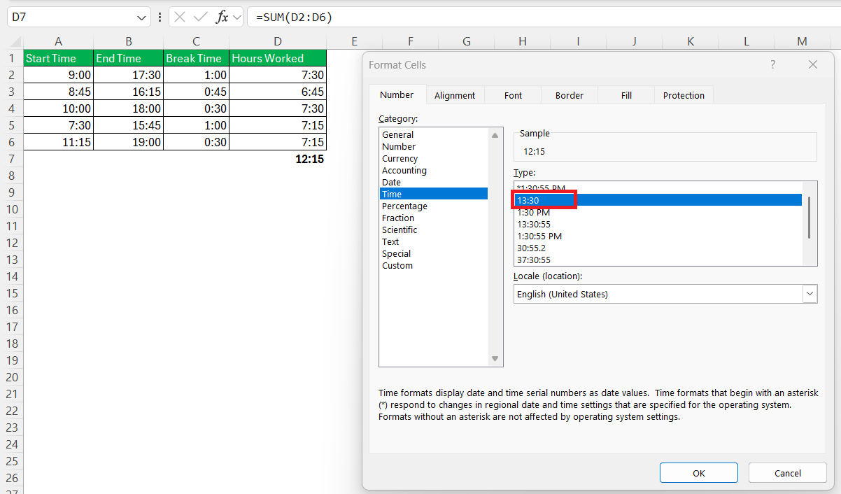
STEP 3: To display the sum correctly as hours exceeding 24, right-click the cell with the total, and choose ‘Format Cells’ > ‘Time’. Select the format hh:mm in the ‘Type’ box. This format allows Excel to display the total as cumulative hours.

Double-check the results against a manual calculation or a smaller sample to ensure that the format and sum are rendering correctly.

By following these steps, you ensure that your total time calculations are accurately presented, even when surpassing 24 hours, providing you with comprehensive insights into the time tracked for projects, events, or activities. This approach is particularly useful for managing continuous operations or multi-day events.

 

FAQs

Why does Excel show strange numbers when I subtract time values?

Excel stores time as a fraction of a 24-hour day. So, if the result isn’t formatted properly, Excel might display it as a decimal or even a date. To fix this, format your result cell using ‘h:mm’ or [h]:mm depending on whether you’re calculating single entries or cumulative hours. This will display the output as a readable time, not confusing numeric values.

What format should I use for cells to calculate and sum time properly?

For individual time differences, use the Time format (h:mm). But when summing hours that exceed 24 (like weekly totals), apply a custom format [h]:mm. The square brackets around h tell Excel not to reset after 24 hours. This ensures your totals reflect actual cumulative hours rather than wrapping around like a clock.

Can Excel handle negative time values (e.g., when someone works past midnight)?

By default, Excel can’t display negative time in standard formats—it shows a series of hash marks (#####) instead. To work around this, either switch to the 1904 date system in Excel’s settings (not recommended for all users), or adjust the time logic to account for overnight shifts using helper columns. Another option is converting to decimal hours for calculations where negative values may occur.

How do I convert hours and minutes into decimal hours for billing purposes?

To convert time into decimal format, multiply the time difference by 24, like this: =((EndTime – StartTime) – BreakTime) * 24. This converts fractions of a day into actual hour values (e.g., 7.5 instead of 7:30). Round it using ROUND(…, 2) for clean billing numbers. This is especially useful when exporting data to accounting software or invoices.

How do I quickly apply these formulas to a whole list of time entries?

Once you’ve written your formula in the first row, use the fill handle (a small square at the bottom-right of the cell) to drag the formula down the entire column. This applies the same logic to all rows, adjusting cell references automatically. Just make sure your time entries are consistent across rows, and you’ll have a complete, calculated list in seconds.