Change Count to Sum in Excel Pivot Tables

How to Change Count to Sum in Pivot Table

Method 1: Use Pivot Table Fields

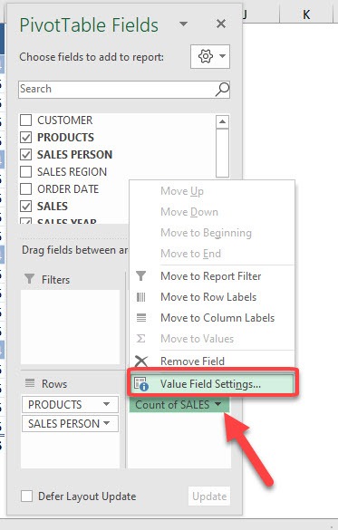
STEP 1: Open the PivotTable fields and click on the arrow beside Count of SALES. In the dropdown, select Value Field Settings.

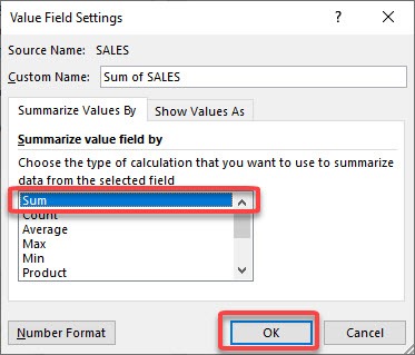
STEP 2: Select Sum and click OK.

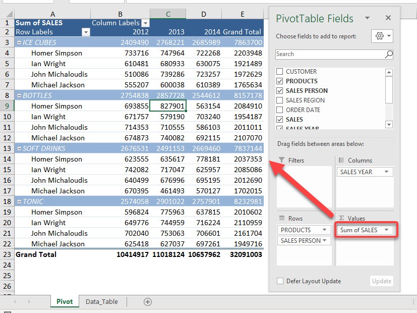
Now your Sales values are being calculated as Sum instead of Count!

Method 2: Use Pivot Table cells

Step 1: Select any cell within the column.

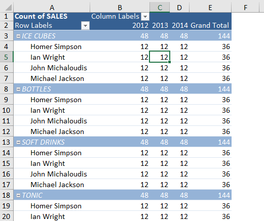
Step 2: Right-click the cell and select Summarize Values By > Sum from the drop-down menu.

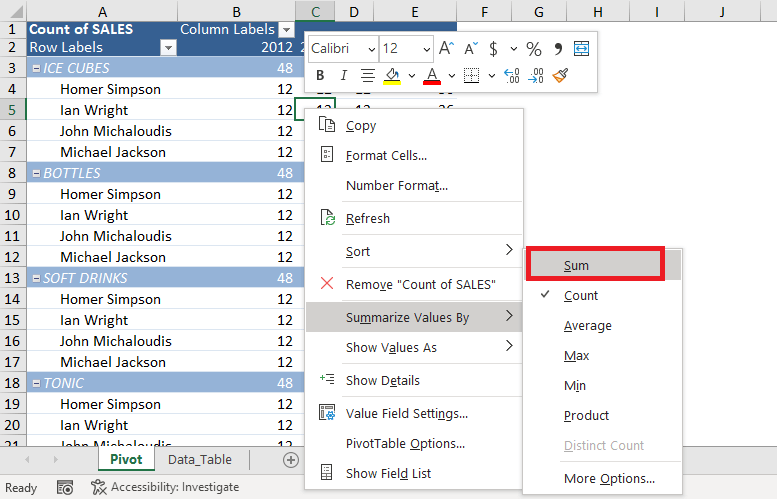
As you can see, the field value has now been updated to SUM instead of COUNT.

 

Troubleshooting Common Pivot Table Sum Issues

Blanks Cells in Source Data

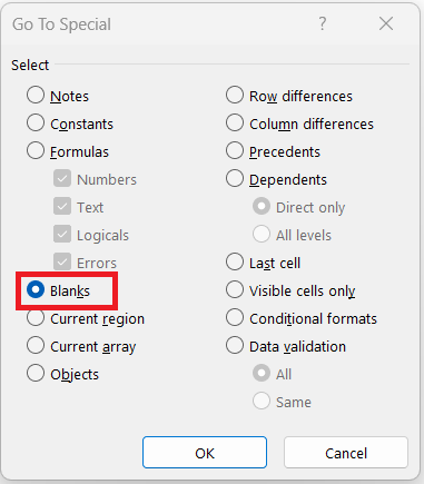
If the Pivot Table shows count instead of sum, it can be because the source data contains blank entries. To fill those blank cells with zero,

• Press Ctrl + R to open Find & Replace
• In Find what box, leave it empty
• In the Replace with box, type 0
• Press Replace All

Errors with Sum Function and How to Address Them

When you encounter errors within your source data, they can cascade into your PivotTable’s sum function, which can be quite the headache. Not to worry though, as you can tackle them with a few clever strategies. If your data fields have errors such as #DIV/0! or #VALUE!, these errors will appear in your PivotTable and corrupt sum totals.

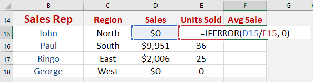
Here’s what you can do: Consider removing or correcting the errors in your source data first. If that’s not possible, try applying the IFERROR function around your formulas to handle errors gracefully. For example, =IFERROR(A2/B2,0) replaces a division error with a zero.

Additionally, adjusting your PivotTable’s settings could help. Opt to use the “Count Numbers” function, which skips errors, text, and blanks, or “Count” which includes errors and numbers for a more accurate representation.

 

Improve Excel Productivity

Create Summary Reports and Dashboards

One of the true strengths of Excel lies in its capability to create succinct, informative summary reports and dashboards from complex datasets. Crafting these high-level perspectives can be greatly simplified with PivotTables. To begin, select the range of data you want to analyze and insert a PivotTable. Then, drag and drop fields into the Rows, Columns, and Values areas to design your report layout. With the Values area, use the sum function for a cumulative analysis of your numeric data.

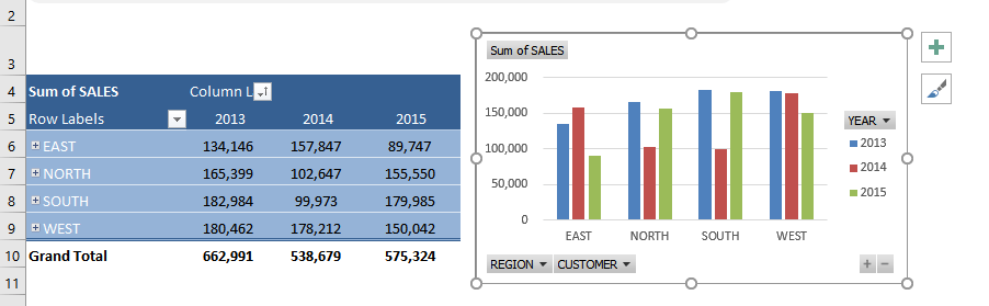
Dashboards elevate your reporting game; they provide an interactive way to visualize key metrics at a glance. By creating a PivotTable, you can then enhance it with PivotCharts, Slicers, and Timelines for a dynamic dashboard that provides insightful analysis and drill-down capabilities.

By changing the design and applying conditional formatting, you can spot important data trends and outliers.

Use Slicers for Data Analysis

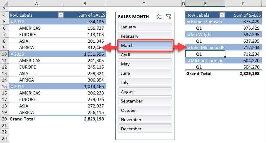
Slicers are a great tool in Excel to examine your data. It can be used to filter the information shown in your PivotTable or PivotChart. To add slicers,

• Click on your PivotTable
• Go to the PivotTable Tools on the ribbon
• Choose the Analyze tab
• Select Insert Slicer
• Select the fields you’d like to use as filters
• With just a click, filter your data

These slicers are customizable, and you can alter the colors, buttons, and settings to make the slicer large or compact.

 

FAQs

1. Why does my Pivot Table show Count instead of Sum?

When the source data contains text, blanks, or numbers stored as text, Excel shows a count of values in the Pivot Table.

2. How to change Count to Sum in a Pivot Table?

To change the count to sum in the Pivot Table,

• Right-click any value in the Pivot Table.
• Select Summarize Values By.
• Click Sum to change the calculation from Count to Sum.

3. What is a Pivot Table?

A Pivot Table is a feature in Excel that helps you to quickly summarize large amounts of data without changing the original dataset.

4. How to refresh the Pivot Table after altering the data?

To refresh a Pivot Table,

• Right-click anywhere in the Pivot Table.
• Select Refresh from the menu.

5. How to use both Count and Sum in the same Pivot Table?

You can use both count and sum in the same Pivot Table by adding the same field twice in the value field. Then, apply different calculations to each field.