Count Text Occurrences with Excel’s SUBSTITUTE Formula

What does it do?

It replaces specific text in a text string i.e. Substitutes new text for old text in a text string.

Formula breakdown:

=SUBSTITUTE(text, old_text, new_text, [instance num])

What it means:

=SUBSTITUTE(This cell, From this TEXT character, To this TEXT character, [In the 1st, 2nd…instance it occurs])

---

I had a scenario where I had to count the number of occurrences of a specific character in a cell.

For example, I had to check the number of asterisks * in a cell.  Why you ask?

Well it was because the asterisks corresponded to the number of times the employee was away that year.  Who would’ve thought of putting asterisks, but there you go!

At first, I had no clue on how to do this and it was very cumbersome to do this manually!

Turns out, the SUBSTITUTE formula in Excel can be used creatively to extract the count easily!

Here’s an example:

We want to return the count of asterisks here, which is 7. We will use a combination of the LEN formula and the  SUBSTITUTE formula.

We will have 3 main steps:

• Get the length of the entire string – in this case, the length of “Bradley Strickland *******” would be 26.
• Get the length of the text without the asterisks – in this case, the length of “Bradley Strickland” would be 19.
• Subtract the two lengths – this will give us 7, which is the number of asterisks.

I explain how you can do this and please go to the bottom of the page to see the animated gif tutorial:

 

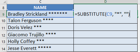
STEP 1: We need to use the SUBSTITUTE function to remove all of the asterisks from the text. We will replace the asterisk “*” with an empty string “”.

=SUBSTITUTE(C9, “*”, “”)

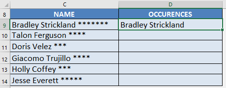
You can see now that the asterisks are removed:

 

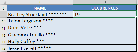
STEP 2: With this result, we can get the length of the text without asterisks using the LEN function:

=LEN(SUBSTITUTE(C9, “*”, “”))

The length of “Bradley Strickland” is 19:

 

STEP 3: Now here is the cool part!

Since we have the length of the text without asterisks, we now get the length of the complete text with asterisks, then we subtract them together. This will give us the number of asterisk occurrences in the text!

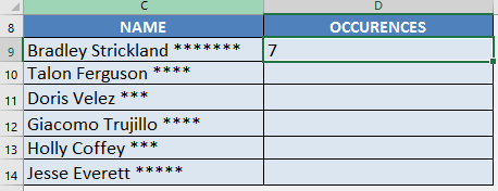
=LEN(C9) – LEN(SUBSTITUTE(C9, “*”, “”))

 

This formula gives us 26 – 19, wherein 26 is the length of the whole text, while 19 is the length of the text without asterisks.

This will give us 7, which is the exact number of asterisks in the text!

 

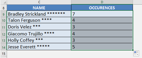
STEP 4: Do the same for the rest of the cells by dragging the SUBSTITUTE formula all the way down using the left mouse button.

Note that all of the counts are automatically calculated: