Disable/Enable Get Pivot Data Using Macros In Excel

If you’ve worked extensively with Pivot Tables in Excel, you’ve probably noticed that whenever you try to reference a cell inside a Pivot Table, Excel doesn’t give you a normal cell reference. Instead, it inserts a GETPIVOTDATA formula automatically. While this formula is extremely powerful for extracting specific data from a Pivot Table, it can be frustrating if all you want is a straightforward reference like =B5 or =C10.

Fortunately, Excel allows you to disable or enable GETPIVOTDATA using a simple macro. This gives you full control over whether Excel automatically generates these formulas when you reference Pivot Table cells.

In this guide, we will go step by step through the process of using Excel Macros to control the GETPIVOTDATA behavior..

Key Takeaways:

• Excel automatically generates GETPIVOTDATA when you reference a Pivot Table cell.
• GETPIVOTDATA is dynamic and extracts specific data from Pivot Tables reliably.
• You can disable or enable GETPIVOTDATA using a simple VBA macro.
• Application.GenerateGetPivotData controls this behavior in Excel.
• Disabling GETPIVOTDATA allows normal cell references, while enabling it ensures dynamic formulas.

 

Exercise Workbook:

 

Understanding GETPIVOTDATA in Excel

What is GETPIVOTDATA?

Before we dive into macros, let’s quickly understand what GETPIVOTDATA is.

GETPIVOTDATA is an Excel function that retrieves specific data from a Pivot Table. Its syntax looks something like this:

=GETPIVOTDATA(“Sales”,$A$3,”Region”,”East”,”Month”,”January”)

Here, Excel extracts the sales value for the East region in January from a Pivot Table located at cell A3.

This function is dynamic. Even if you move the Pivot Table or change its layout, GETPIVOTDATA still references the correct data. While this is excellent for dynamic reporting, it can be annoying if you just want a simple formula pointing to a specific cell.

Why Disable GETPIVOTDATA?

Disabling GETPIVOTDATA is useful when:

• You are creating formulas referencing Pivot Table data and don’t want Excel to generate complex GETPIVOTDATA formulas.
• You want simpler, direct cell references for easier readability and editing.
• You are preparing a report where GETPIVOTDATA formulas could confuse collaborators.

Enabling it back is useful when:

• You want to make your formulas dynamic and robust.
• You want Excel to automatically update references even if the Pivot Table changes.

 

Disable/Enable Get Pivot Data Using Macros

Enable Developer Tab

Before you can create a macro, you must ensure that the Developer tab is visible in Excel. Here’s how:

STEP 1: Go to File > Options.

STEP 2: Click Customize Ribbon.

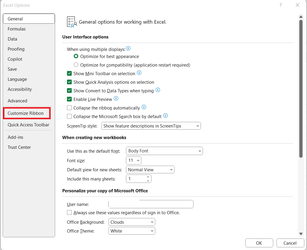
STEP 3: In the right-hand panel, check Developer. Click OK.

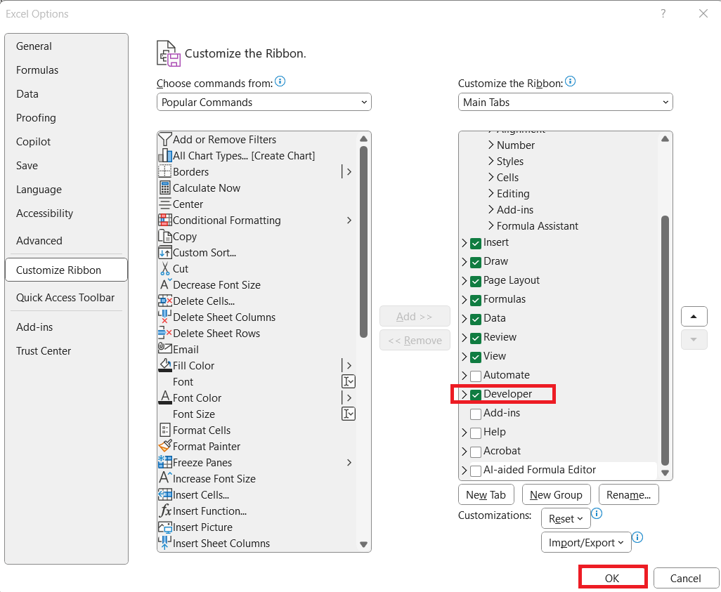
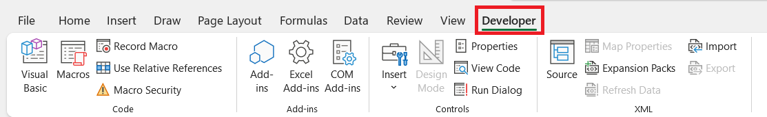
Once the Developer tab is enabled, you can access the Visual Basic Editor to write macros.

Write VBA Code: Step-by-Step Guide

Here is our pivot table:

If we try to create a formula involving one of the cells inside the Pivot Table, you will see the GETPIVOTDATA Formula. Let us change this behavior using Macros!

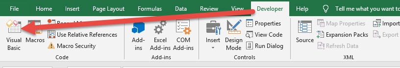
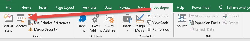
STEP 1: Go to Developer > Code > Visual Basic

STEP 2: Paste in your code and Select Save. This will create two options for you to choose either to enable or to disable. Close the window afterwards.

Sub EnableGetPivotData()
Application.GenerateGetPivotData = True
End Sub
Sub DisableGetPivotData()
Application.GenerateGetPivotData = False
End Sub

STEP 3: Let us test it out!

Open the sheet containing the data. Go to Developer > Code > Macros

Make sure your disabled macro is selected. Click Run.

Try referencing a cell inside the pivot table again. It is now a normal cell reference. With just one click, we have disabled get pivot data!

 

Explanation of the code

Application.GenerateGetPivotData is a property in Excel that controls GETPIVOTDATA behavior.

• Setting it to True enables GETPIVOTDATA.
• Setting it to False disables it.

After pasting the code, save your workbook as a macro-enabled file (.xlsm) to retain the macros.

 

Tips for Using This Macro

• Save Your Work: Always save your Excel file before running macros, especially if you’re disabling GETPIVOTDATA in a large workbook.
• Macro Security: Make sure your macro security settings allow running macros. Go to File > Options > Trust Center > Trust Center Settings > Macro Settings.
• Shortcut Key: You can assign a shortcut key to your macro for quick access. In the Macros dialog, select the macro, click Options, and set a key combination.
• Test in a Sample File: Before applying macros to your main workbook, test on a copy to avoid unintended changes.

 

FAQs

1. What is GETPIVOTDATA in Excel?

GETPIVOTDATA is an Excel function that retrieves specific data from a Pivot Table. It allows you to reference values dynamically, even if the Pivot Table layout changes. For example, it can pull sales for a specific region and month using a structured formula. While very useful for dynamic reporting, it can be cumbersome if you just want a normal cell reference. You can control this behavior using macros to enable or disable it.

2. Why would I want to disable GETPIVOTDATA?

Disabling GETPIVOTDATA is helpful when you prefer simple, direct cell references. It makes formulas easier to read and edit, especially for users unfamiliar with complex Pivot Table formulas. It’s also useful when preparing reports for collaborators who might find GETPIVOTDATA confusing. Disabling it does not affect the Pivot Table itself. You can re-enable it anytime if you need dynamic references.

3. How do I enable or disable GETPIVOTDATA using a macro?

First, ensure the Developer tab is enabled in Excel. Then, open the Visual Basic Editor, insert a module, and paste the macro code. Use Application.GenerateGetPivotData = False to disable or = True to enable it. After saving your workbook as a macro-enabled file (.xlsm), go to Developer > Macros and run the desired macro. Once executed, referencing a Pivot Table cell will follow your chosen setting.

4. Do I need to save my workbook before running these macros?

Yes, it’s recommended to save your workbook before running macros, especially in large files. Macros make changes to Excel’s behavior, so saving ensures you can revert if something goes wrong. Always use a macro-enabled format (.xlsm) to retain the code. It’s also smart to test macros in a sample workbook first. This prevents accidental data or formula errors.

5. Can I automate enabling/disabling GETPIVOTDATA for a specific worksheet?

Yes, you can attach VBA code to worksheet events. For example, Worksheet_Activate can automatically disable GETPIVOTDATA whenever that sheet is opened. Similarly, you can enable it when switching to another sheet. This approach avoids manually running macros each time. It’s ideal for reports that require different Pivot Table behaviors across worksheets.