Filter by Text wildcards

Pivot Table allows you to filter by text wildcard characters and make your filtering dynamic. You can use the row label filter and enter the text with wildcards to get the desired result.

Wildcards can take place of any character and the two wildcards that you can use while filtering text in Pivot Table is:

• Asterisk (*) – This returns any series of characters before or after the asterisk
• Question Mark (?) – This returns text that contains one variable

Key Takeaways

• Wildcards Simplify Complex Filters – Excel supports the use of * (asterisk) and ? (question mark) to filter and match patterns in text data.

• Asterisk Matches Multiple Characters – Use * when you want to match any number of characters. For example, *Report will return all entries that end with “Report”.

• Question Mark Matches a Single Character – Use ? to match exactly one character. For example, R?in matches “Rain”, “Ruin”, and “Rhin”.

• Works in Filters, Search, and Formulas – Wildcards are not just for filtering; they also work with functions like COUNTIF, SUMIF, and SEARCH.

• Case-Insensitive Matching – Wildcard filters in Excel are not case-sensitive, making them user-friendly for quick lookups and summaries.

The Multiple Scenarios for Wildcards

You can check out the multiple scenarios here:

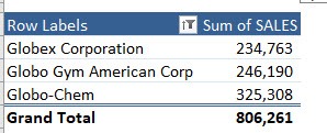
• When you add * after Glo, Excel will filter cells that contain text starting with Glo like Globex Corporation, Globo Gym American Corp, etc.
• When you add * before tech, Excel will filter cells that contain text ending with tech like Initech, Primatech, etc.
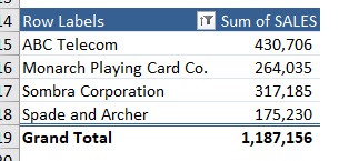
• When you add ? in between a and c, Excel will filter data and containers any one character in between a and c. For example – ABC Telecom, Monarch Playing Card Co, etc.

 

How to Filter by Text wildcards

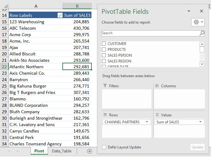
This is our current Pivot Table setup. Let us see how these filter by text wildcards work!

 

Example 1: Use Asterisk (*)

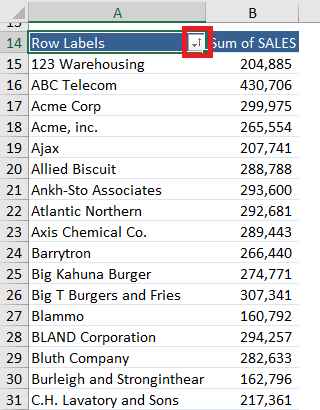
STEP 1: Click on the Row Label filter button in the Pivot Table.

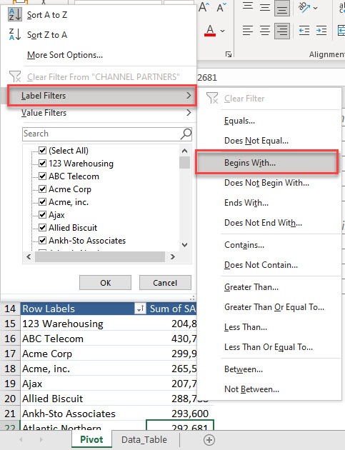
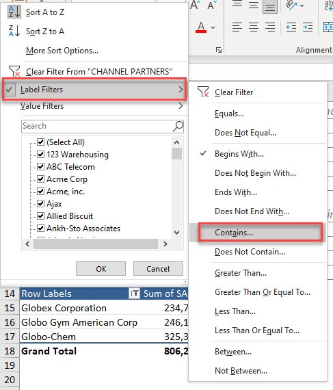
STEP 2: Select Label Filters.

You will see that we have a lot of filtering options. Let us try out Begins With

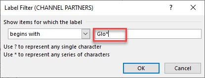
STEP 3: Type in Glo*

This will give us all the channel partners that start with Glo, what comes after that doesn’t matter.

Click OK

And you have the values starting with Glo!

 

Example 2: Use Question Mark (?)

STEP 1: Click on the Row Label filter button in the Pivot Table.

STEP 2: Select Label Filters > Contains

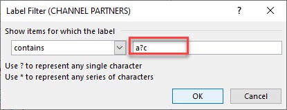
STEP 3: Type in a?c in the Label Filter dialog box.

This will give us all the channel partners that have a<any character>c inside.

Click OK

You can see it matched “abc”, “arc” and “a c”

This is how you can make filtering in Pivot Table handy by using filter by text wildcard!

Frequently Asked Questions

What are the wildcard characters in Excel?
Excel uses two main wildcards: * (matches any number of characters) and ? (matches a single character).

Can I use wildcards in Excel’s filter dropdown menu?
Yes, just go to the filter search box and type your wildcard text (e.g., *summary*), and Excel will filter matching values.

How do I filter for values that begin with a specific word?
Use word* in the filter box or in a formula like =COUNTIF(A1:A100, "word*") to match values that start with “word”.

Can wildcards be used with conditional formatting?
Yes, formulas with wildcards (like =ISNUMBER(SEARCH("*error*", A1))) can be used to apply conditional formatting based on partial text matches.

What if I want to search for an actual asterisk or question mark?
Use a tilde ~ before the character. For example, ~* searches for a real asterisk, and ~? searches for a question mark.