FIND Formula in Excel

If you’ve ever tried to locate a specific character or word inside a longer string of text in Excel, you’ve probably done a lot of squinting, scrolling, and mumbling under your breath. But there’s a far cleaner, smarter, and faster way to pinpoint exactly where that text appears — and that’s with the FIND function.

This formula is one of Excel’s simplest yet most powerful text functions. It’s like having a mini detective living inside your spreadsheet, ready to tell you exactly where a word, letter, or character is hiding.

Let’s dive deep and unpack this little gem.

Key Takeaways:

• The FIND function helps you locate the position of a specific character or word inside another text string.
• It is case-sensitive, meaning “X” and “x” are treated as different characters.
• The syntax is =FIND(find_text, within_text, [start_num]), where the third argument is optional.
• When the text isn’t found, Excel returns a #VALUE! error, which can be handled using IFERROR.
• FIND becomes even more powerful when combined with other text functions like LEFT, RIGHT, and MID.

 

Understanding the FIND Formula

What Does the FIND Function Do?

The FIND formula helps you get the position of specific text within another text. In plain English, if you have the word “Excel” and you want to know where the letter “x” appears, FIND will tell you it’s the second character in the word.

For instance:

=FIND(“x”, “Excel”)

This will return 2, because the letter “x” appears in the second position of “Excel”. Pretty simple, right? But as you’ll soon see, FIND can do a lot more when combined with other formulas.

FIND Formula Syntax

Here’s the syntax:

=FIND(find_text, within_text, [start_num])

• find_text – The text or character you want to search for.
• within_text – The cell or text string where you want to search.
• start_num (optional) – The position in the source text where you want to start the search. Default is 1 (meaning it starts from the beginning).

 

Step-by-Step Guide: Detailed Examples

Example 1: Find Formula

STEP 1: We need to enter the FIND function in a blank cell:

=FIND(

STEP 2: The FIND arguments:

find_text

What is the text to be searched for?

Select the cell containing the text to be searched for. In our first example, we want to search for ‘x’ in the word ‘Excel’:

=FIND(D9,

within_text

What is your source text?

Select the cell source text. So let’s select ‘Excel’ as our source text:

=FIND(D9, C9,

start_num

Where do you want to start searching in your source text?

You can leave this blank; it will default to 1, which means it will start looking from the first character of your source text. In our case, let us put in 1 to start searching from there:

=FIND(D9, C9, 1)

Apply the same formula to the rest of the cells by dragging the lower right corner downwards.

You can see that the matching is case sensitive! And if it’s unable to find your text, it will return #VALUE.

 

Example 2: FIND + MID for Extracting Text Dynamically

You can combine FIND with the MID function to extract a specific portion of text. For example, if you have “Product123” and want to extract the numbers after “Product”, use:

=MID(A1, FIND(“t”, A1) + 1, LEN(A1))

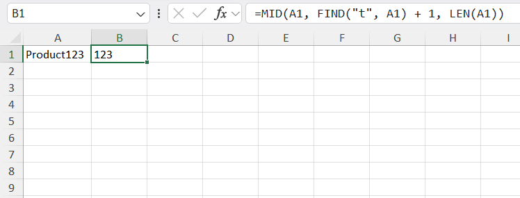
This formula finds where “t” ends, moves one character forward, and extracts the rest of the text. The result is “123”.

Example 3: FIND + LEFT and RIGHT for Splitting Text

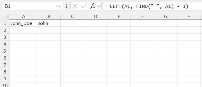
If you have a full name like “John_Doe” and want to split it into first and last names:

=LEFT(A1, FIND(“_”, A1) – 1)

=RIGHT(A1, LEN(A1) – FIND(“_”, A1))

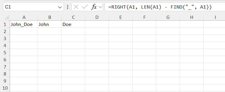
These formulas locate the underscore and separate the text accordingly, giving you “John” and “Doe”.

 

Handling #VALUE! Errors

Whenever the text isn’t found, the FIND function returns the #VALUE! error. This usually happens for a few common reasons:

• The search text doesn’t exist in the source.
• The case doesn’t match.
• The start position is beyond the length of the text.

To fix or handle this, use:

=IFERROR(FIND(“X”, “Excel”), “Not Found”)

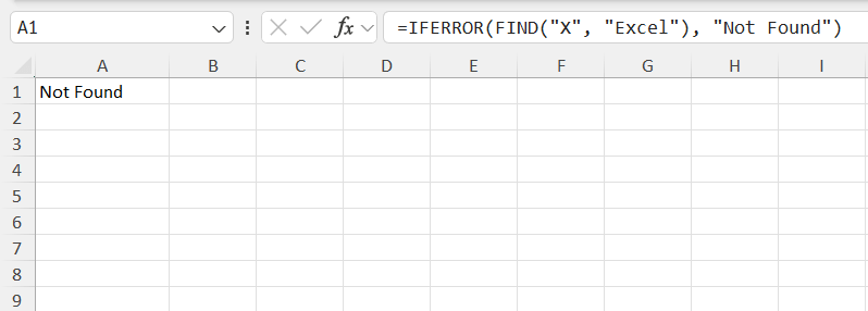
That way, your formula doesn’t break — it just tells you the result nicely.

 

FAQs

1. What is the difference between FIND and SEARCH in Excel?

The FIND and SEARCH functions both locate text within another text, but the key difference is case sensitivity. FIND is case-sensitive, so “A” and “a” are treated differently, while SEARCH ignores case differences. For example, =FIND(“A”, “apple”) returns an error, while =SEARCH(“A”, “apple”) returns 1. If you need strict matching, use FIND; if you prefer flexibility, use SEARCH. Both can be combined with other text functions for even more control.

2. What happens when the text is not found using FIND?

When Excel cannot locate the specified text, it returns a #VALUE! error. This indicates that the searched text doesn’t exist in the source string or that there’s a case mismatch. It may also occur if your starting position is greater than the total number of characters in the text. To avoid breaking your formulas, wrap FIND inside IFERROR or ISNUMBER. This way, you can display “Not Found” or another custom message instead of an error.

3. Can FIND locate multiple occurrences of the same character?

By default, FIND only identifies the first occurrence of a text or character. However, you can use the start_num argument to find subsequent ones. For example, =FIND(“e”, “Excel Excel”, 3) starts the search from the third character, helping you locate the second “E”. For dynamic multiple matches, you’ll need to combine FIND with other functions like MID, SUBSTITUTE, or even use array formulas. This lets you analyze repeating characters or patterns efficiently.

4. How can I make FIND case-insensitive?

Since FIND is naturally case-sensitive, you can’t disable this feature directly. Instead, use the SEARCH function, which works the same way but ignores letter case. For example, =SEARCH(“x”, “Excel”) and =SEARCH(“X”, “Excel”) both return 2. Alternatively, you can convert both texts to a common case using UPPER or LOWER, such as =FIND(LOWER(“X”), LOWER(“Excel”)). This ensures consistent results regardless of capitalization.

5. How can I handle errors in FIND results gracefully?

Handling errors in FIND is best done using the IFERROR function. This prevents ugly #VALUE! messages from showing up in your report or dashboard. For instance, =IFERROR(FIND(“x”, A1), “Not Found”) replaces the error with a custom message. You can also use IF(ISNUMBER(FIND(“x”, A1)), “Found”, “Not Found”) to display a friendly response. This makes your spreadsheet more user-friendly and visually clean.