Table of Contents
How To Make Negative Red Numbers In Excel
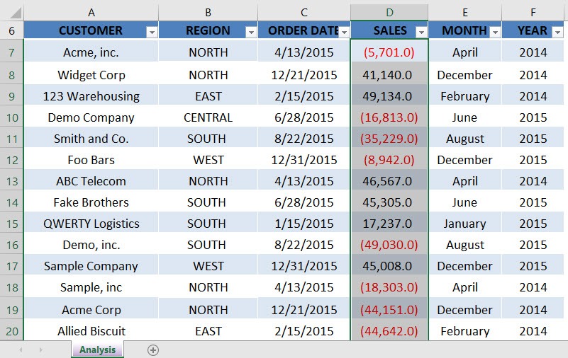
When you are working with lots of different numbers in Excel, you sometimes want your numbers to stand out by showing them in a negative red number enclosed in parenthesis.
To do this you need to select your numbers and press CTRL+1 to bring up the Format dialogue box.
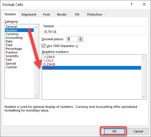
From there you need to select the Number tab and the Number category and choose the 4th selection (1,234.0)
You can then select the number of decimal places to show and also insert a 1000 separator.
Download workbookNumber-Formats-Negatives.xlsx
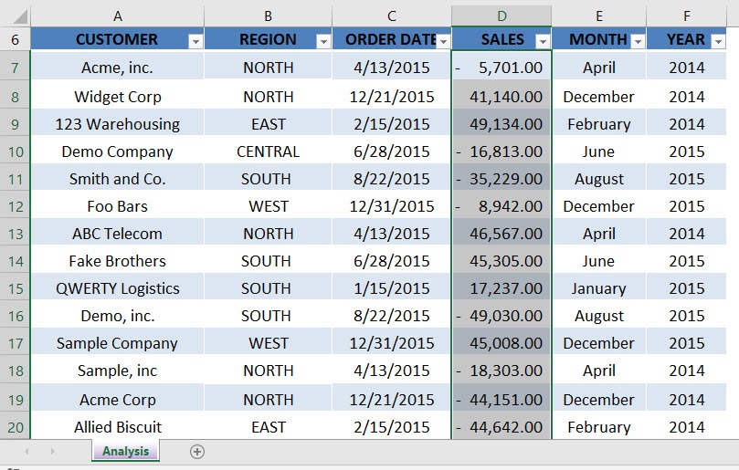
STEP 1: Select the column that you want to apply the negative number formatting. Press CTRL + 1 to open the Format Dialog.
STEP 2: Select Number as the category and select the formatting that you want to display for negative numbers. You can change the number of decimal places as well.
Click OK.
Now your negative numbers are now formatted!
John Michaloudis is a former accountant and finance analyst at General Electric, a Microsoft MVP since 2020, an Amazon #1 bestselling author of 4 Microsoft Excel books and teacher of Microsoft Excel & Office over at his flagship MyExcelOnline Academy Online Course.


