How to Unfreeze Panes in Excel – Step by Step Guide

Microsoft Excel is a powerful tool many of us rely on for data analysis and organization. Among its myriad features, the ability to freeze and unfreeze panes stands out, especially when working with large datasets. I’ve often encountered situations where these features help manage the visibility of crucial data as I scroll. In this guide, I’ll walk you through the simple steps on how to unfreeze panes in Excel, ensuring that navigation through your spreadsheets remains seamless and efficient.

Key Takeaways:

• Unfreezing panes restores full visibility of your Excel sheet, which is helpful when analyzing large datasets.
• It’s quick and easy — just go to the View tab > Freeze Panes > Unfreeze Panes.
• Keyboard shortcut Alt + W + F + F offers a fast, no-mouse-needed way to unfreeze.
• Grayed-out unfreeze options often mean there’s nothing currently frozen or the worksheet is protected.
• Efficient sheet navigation relies on smart pane management and using Excel shortcuts.

 

Why Unfreeze Panes in Excel?

Common Scenarios Requiring Unfreeze

Unfreezing panes in Excel is commonly required when working with dynamic datasets that frequently change in structure or size. For instance, if I’ve previously frozen panes to maintain visibility of header rows or columns and now need a full view of new data, unfreezing becomes essential.

Another scenario might involve collaborating with colleagues who require different views of the workbook, necessitating frequent shifts between frozen and unfrozen states. Additionally, unfreezing is often needed during formatting or when a comprehensive data overview is required for analysis or presentation. These scenarios highlight the need to fluidly switch between frozen and unfrozen states in Excel.

Benefits of Unfreezing Panes

Unfreezing panes in Excel offers several key advantages, primarily revolving around increased flexibility and enhanced data visibility. By unfreezing panes, I can easily view entire spreadsheets without being restricted to fixed rows or columns, which is crucial when analyzing extensive datasets.

This capability allows a seamless examination of data from different perspectives, facilitating comprehensive insights. It also enhances collaboration by simplifying the process of adjusting views for various users or presentations. Unfreezing panes ensures that navigating through data is straightforward and less cumbersome, making the task more efficient and less error-prone.

 

How to Unfreeze Panes in Excel

Using the Menu Options

To unfreeze panes using the menu options in Excel, I start by clicking the “View” tab found on the Ribbon. Within this tab, there is a section called “Window” where I locate the “Freeze Panes” button. If any panes are currently frozen, selecting this button opens a dropdown menu.

Here, I simply choose “Unfreeze Panes” to release the locked rows or columns.

This menu-driven approach is user-friendly, providing me with clear options and ensuring that I can easily switch between different view settings without any hassle. It’s a simple yet effective method for managing how data is displayed.

Keyboard Shortcuts for Efficiency

For those like me who appreciate speed and efficiency, using keyboard shortcuts to unfreeze panes in Excel is a game-changer. To efficiently unfreeze panes, I can use the Alt key in combination with specific shortcuts. I press Alt followed by W, then F, and finally F again.

This sequence mirrors the navigation through the Ribbon menu, targeting the “Freeze Panes” option, and swiftly unfreezing any frozen sections. This method is particularly useful for those who handle a multitude of tasks in Excel and desire a fast, interruption-free workflow.

Use VBA to Unfreeze Panes in Excel

STEP 1: Press Alt + F11 to open the VBA Editor.

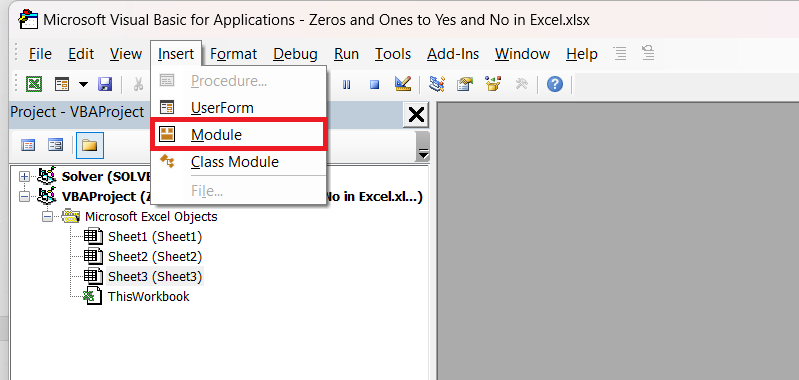
STEP 2: In the editor, go to the Insert menu and click Module.

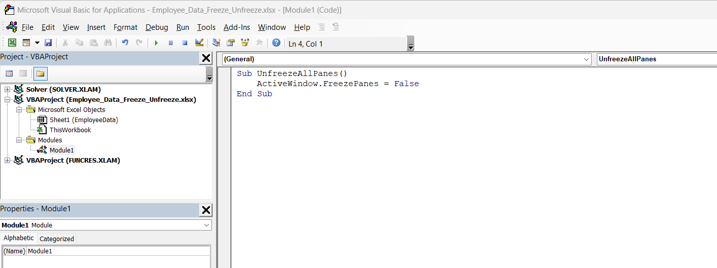
STEP 3: In the new code window, copy and paste the following VBA code:

Sub UnfreezeAllPanes()
ActiveWindow.FreezePanes = False
End Sub

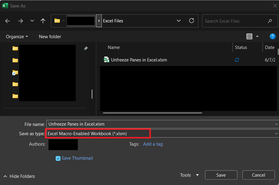
STEP 4: Press Ctrl + S to save your workbook. Make sure to save it as an Excel Macro-Enabled Workbook (.xlsm)

STEP 5: Close the VBA Editor by pressing Alt + Q.

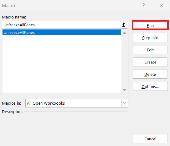
STEP 6: Press Alt + F8 to open the Macro dialog box. Select UnfreezeAllPanes from the list and click Run.

 

Troubleshooting Common Issues

Pane Not Responding

If I encounter a situation where the Excel pane is not responding as expected, a few troubleshooting steps can be beneficial. First, I try refreshing the workbook by closing and reopening it, which often resolves minor glitches. It’s also important for me to ensure that my Excel and system updates are current, as outdated software can cause responsiveness issues.

Checking for any add-ins that might conflict with the pane functionalities can also help. If the problem persists, restarting the computer or opening the workbook in a different Excel version may provide a resolution. In many cases, these steps can restore normal functionality to the panes.

Unfreeze Options Grayed Out

When I find that the “Unfreeze Panes” option is grayed out, it typically indicates a few potential issues. First, I ensure that I am in the correct worksheet, as this feature might not be active if the workbook is protected or in a different view mode. To resolve this, I’ll check if the worksheet is protected by going to the “Review” tab and clicking “Unprotect Sheet” if necessary.

It’s also possible that no panes are actually frozen. Verifying this requires confirming that I’m not trying to unfreeze what hasn’t been frozen in the first place. Checking these elements usually resolves the issue promptly.

Restoring Default View Settings

To restore default view settings in Excel, I begin by ensuring I’m in the worksheet where I want to make the changes. Next, I access the “View” tab in the Ribbon. Here, I select Normal” if I’ve altered the window arrangement and wish to return to the standard layout.

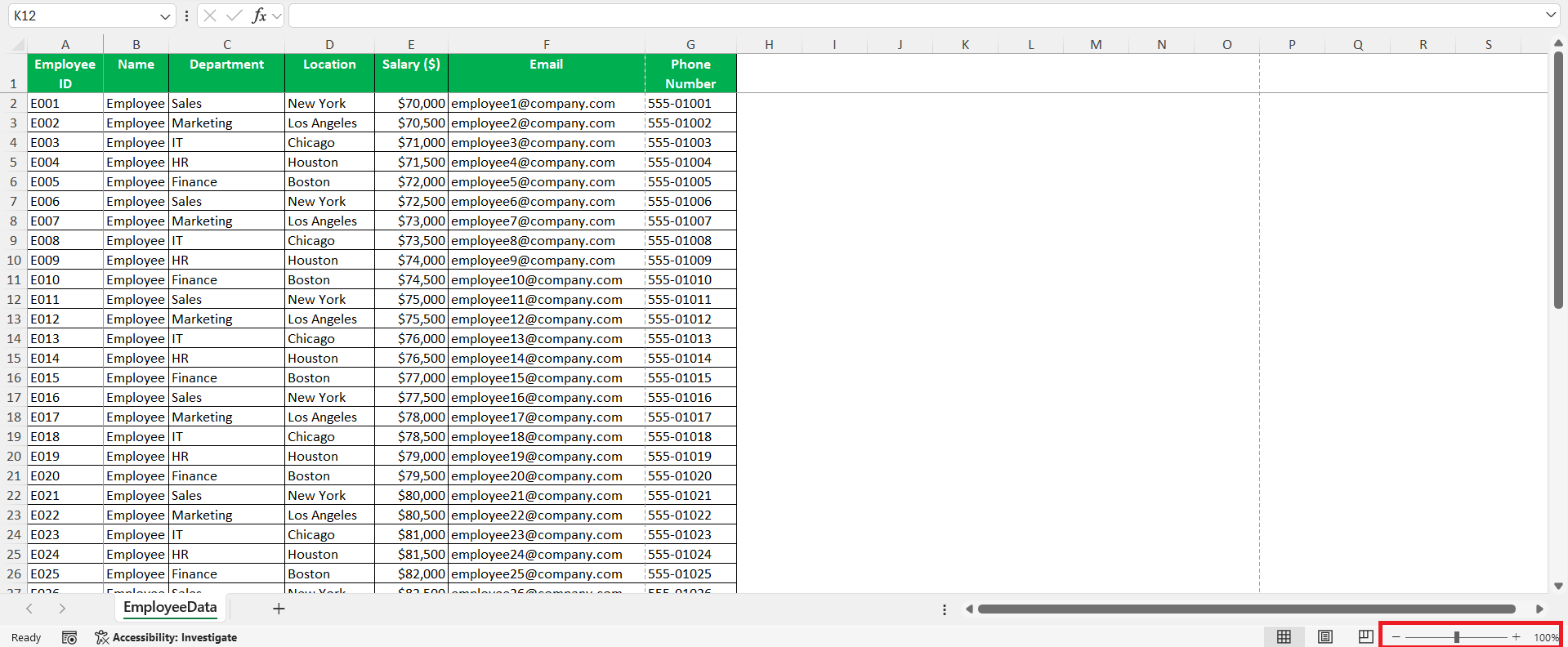
For a more comprehensive reset, deselect any “Freeze Panes” options and switch to the “Normal” view. This ensures rows and columns are no longer fixed, providing a full view of the spreadsheet. Additionally, I can remove any zooming adjustments by resetting the zoom level to 100% using the zoom control slider.

These steps effectively restore an uncluttered and standard workbook view.

 

Best Practices for Efficient Navigation

Efficient navigation in Excel is vital for productivity, and I’ve gathered a few best practices over time. Firstly, I consistently utilize the “Freeze Panes” feature strategically, opting to lock rows or columns that contain critical labels or data identifiers. This ensures they remain visible during extensive scrolling. Additionally, I’m a fan of using keyboard shortcuts for quick movement, such as Ctrl + Arrow keys to jump across data arrays and Ctrl + Home to return instantly to the top-left cell.

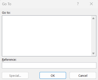
Another practice involves setting up a well-structured worksheet with consistent labeling and formatting, which inherently simplifies navigation. I also make use of the “Go To” feature (by pressing F5 or Ctrl + G) to swiftly jump to any specific cell, facilitating faster access to different parts of the sheet

Lastly, keeping my workbooks uncluttered by avoiding unnecessary freezing and ensuring hidden rows or columns are minimized can further streamline movement through spreadsheets. Through these strategies, I maintain an efficient and organized approach to managing and navigating my Excel workbooks.

 

FAQs

Why would I need to unfreeze panes in Excel?

You may need to unfreeze panes when your dataset has changed, making frozen headers or columns irrelevant or obstructive. It’s also necessary when sharing files with others who prefer different views, or when preparing the sheet for printing or presentations. Unfreezing allows you to view the full spreadsheet without restrictions. This improves flexibility and makes reviewing large data sets easier.

What happens when you unfreeze panes in Excel?

Unfreezing panes in Excel restores the worksheet to its default scrolling behavior, allowing all rows and columns to move freely. This action removes any fixed rows or columns, enabling me to navigate the entire dataset without restrictions, enhancing my ability to view the complete range of data.

Can I refreeze panes after unfreezing them?

Yes, you can refreeze panes after unfreezing them in Excel. Simply navigate to the “View” tab in the Ribbon, and choose “Freeze Panes.” From there, you can select the appropriate freeze option to reapply the freeze to your chosen rows or columns, allowing customization for your data viewing needs.

Why can’t I unfreeze the panes in my workbook?

If you’re unable to unfreeze panes in your workbook, it may be due to worksheet protection, causing the option to be inaccessible. Also, ensure that the workbook is in “Normal” view, not in “Page Break Preview” or another mode, as this can affect your ability to modify pane settings.

Can I use a keyboard shortcut to unfreeze panes?

Yes! You can quickly unfreeze panes using the keyboard by pressing Alt → W → F → F. This sequence mimics the Ribbon navigation and saves time for power users. It’s especially useful if you handle large datasets often and want to avoid extra clicks. This method works consistently across Excel versions.