How to Use SUMIFS Function in Excel

To fully utilize Excel’s capabilities as a tool for managing data, it’s crucial to have a solid grasp of all of its features. The SUMIFS function, which enables you to sum values in a range that satisfies multiple conditions, is one such function.

When you need to analyze data depending on many criteria, the SUMIFS function comes in handy. It is a flexible function that may be applied in a wide range of situations, from determining sales numbers for particular goods or geographical areas to examining client information based on demographics or purchase patterns.

SYNTAX

=SUMIFS(Sum_Range,Criteria_Range1,Criteria1,Criteria_Range2,Criteria2…)

• Sum_Range (required) – The range of cells to sum.
• Criteria_Range1 (required) – The range that is tested using Criteria1. Criteria_range1 and Criteria1 set up a search pair whereby a range is searched for specific criteria. Once items in the range are found, their corresponding values in Sum_range are added.
• Criteria1 (required) – The criteria that define which cells in Criteria_range1 will be added. For example, criteria can be entered as 32, “>32”, B4, “apples”, or “32”.
• Criteria_Range2, Criteria2, … (optional) – Additional ranges and their associated criteria.

You can enter up to 127 range/criteria pairs.

Let us look at a few examples to help us understand this function better.

Download the Excel Workbook below to follow along and understand how to highlight duplicates in Excel –

download excel workbookSUMIFS-in-Excel.xlsx

 

Example 1

In this example, we are looking up the total sales amount for product 1001 in the East region. Let us understand it with the help of a step-by-step tutorial.

STEP 1: Enter the SUMIFS function in cell F3.

=SUMIFS(

STEP 2: Enter the first argument – Sum_range. Here we have selected the range C2:C89 as it contains all the sales figures.

=SUMIFS(C2:C89,

STEP 3: Enter the second argument – Criteria_range1. Here we have selected B2:B89 range as it contains the region of sale details. We will apply our East region criteria in this range.

=SUMIFS(C2:C89,B2:B89,

STEP 4: Enter the third argument – Criteria1. Here we have entered “East” as we want the sum of sales in the East region.

=SUMIFS(C2:C89,B2:B89,”East”,

STEP 5: Enter the fourth argument – Criteria_range2. Here we have selected A2:A89 range as it contains the product ID details. We will apply our product 1001 criteria in this range.

=SUMIFS(C2:C89,B2:B89,”East”,A2:A89,

STEP 6: Enter the fifth argument – Criteria2. Here we have entered “1001” as we want the sum of sales of product 1001.

=SUMIFS(C2:C89,B2:B89,”East”,A2:A89,”1001″)

As we can see, the SUMIFS function returns the sum of sales of product 1001 in the East region, applying multiple criteria at once.

 

Example 2

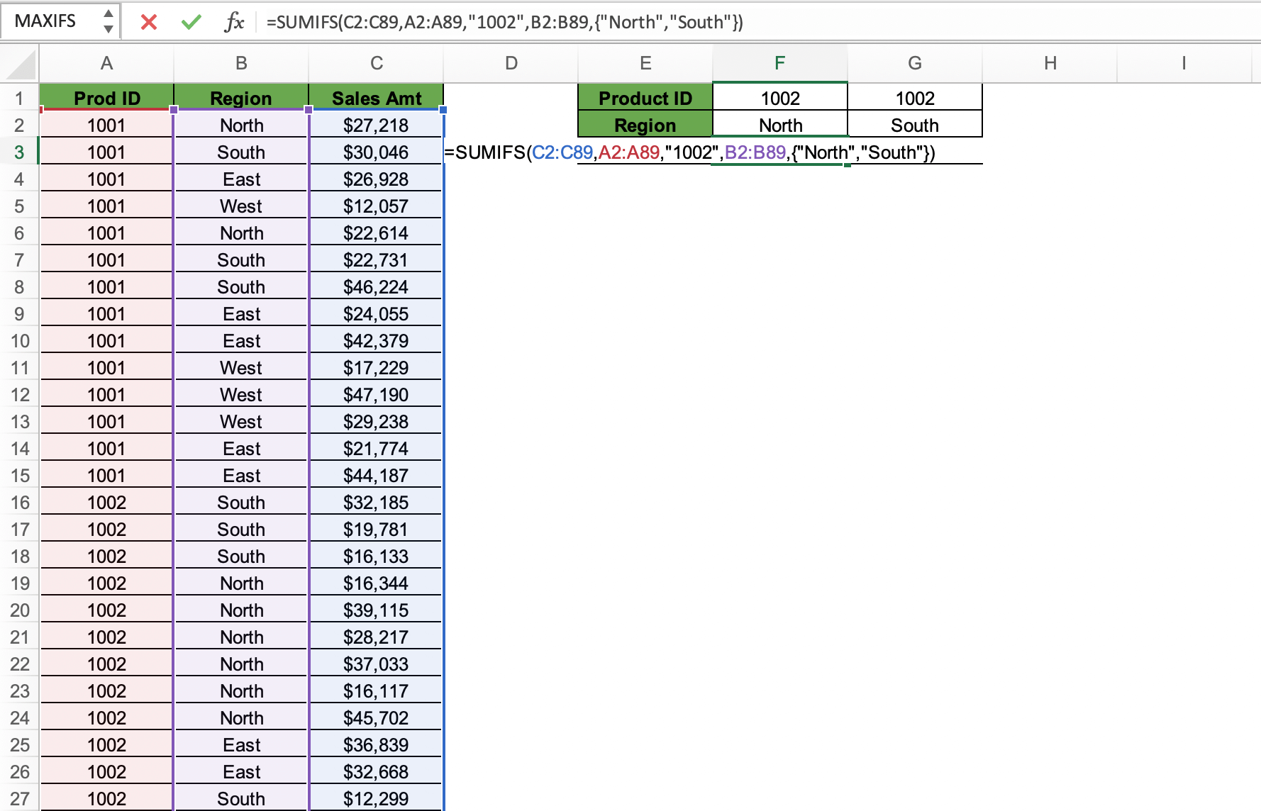
Here we will find the sales for product 1002 in the north and south region in cells F3 and G3. Let’s understand this step by step

STEP 1: Enter the SUMIFS function in cell F3.

=SUMIFS(

STEP 2: Enter the first argument – Sum_range. Here we have selected C2:C89 range as it contains all the sales figures of which we want the sum.

=SUMIFS(C2:C89,

STEP 3: Enter the second argument – Criteria_range1. Here we have selected A2:A89 range as it contains the product ID details. We will apply our product 1002 criteria in this range.

=SUMIFS(C2:C89,A2:A89,

STEP 4: Enter the third argument – Criteria1. Here we have entered “1002” as we want the sum of sales of product 1002.

=SUMIFS(C2:C89,A2:A89,”1002″,

STEP 5: Enter the fourth argument – Criteria_range2. Here we have selected B2:B89 range as it contains the region of sale details. We will apply our North and South criteria in this range.

=SUMIFS(C2:C89,A2:A89,”1002″,B2:B89,

STEP 6: Enter the fifth argument – Criteria2. Here we have entered {“North”, “South”} as we want the sum of sales in the regions North and South separately in cells F3 and G3.

=SUMIFS(C2:C89,A2:A89,”1002″,B2:B89,{“North”,”South”})

Make sure to keep your criteria in curly brackets.

As we can see, the SUMIFS function returns the sum of sales of product 1002 in North and South regions, applying multiple criteria at once.

This can also be achieved if we used 2 SUMIFS functions separately as we did in our first example.

 

Example 3

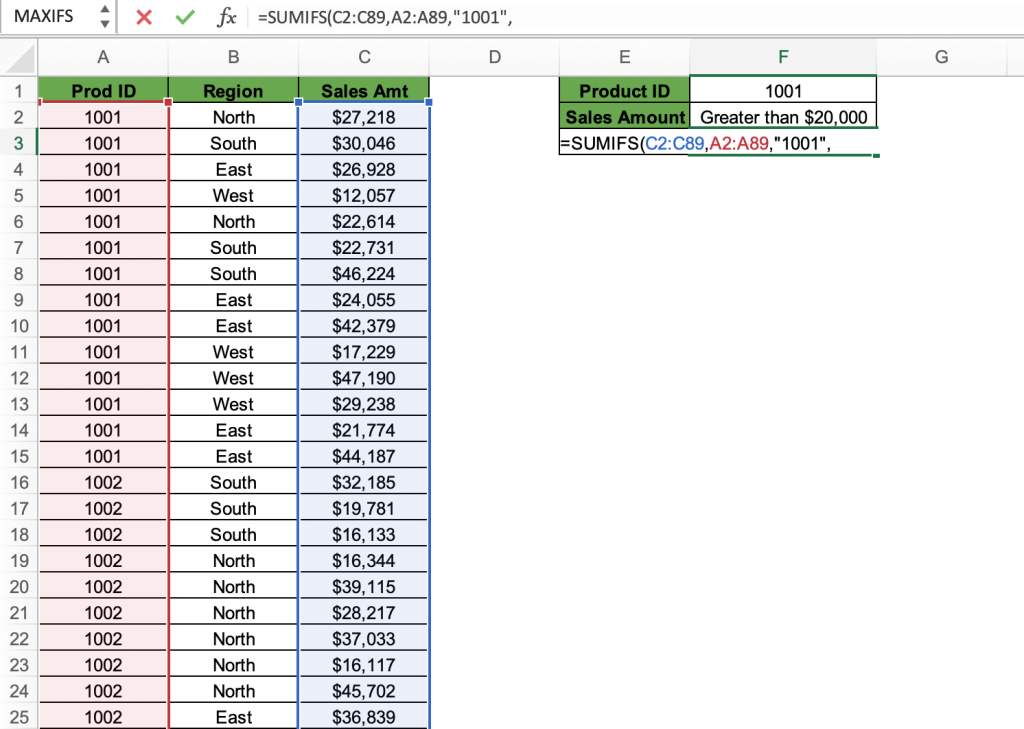
In this example, we are looking up the total sales amount for product 1001 but only when the sales amount is greater than $20,000.

STEP 1: Enter the SUMIFS function in cell F3.

=SUMIFS(

STEP 2: Enter the first argument – Sum_range. Here we have selected C2:C89 range as it contains all the sales figures of which we want the sum.

=SUMIFS(C2:C89,

STEP 3: Enter the second argument – Criteria_range1. Here we have selected A2:A89 range as it contains the product ID details. We will apply our product 1002 criteria in this range.

=SUMIFS(C2:C89,A2:A89,

STEP 4: Enter the third argument – Criteria1. Here we have entered “1001” as we want the sum of sales of product 1001.

=SUMIFS(C2:C89,A2:A89,”1001″,

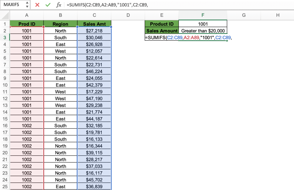
STEP 5: Enter the fourth argument – Criteria_range2. Here we have selected range C2:C89 as it contains the sales amount. We will apply the rule – greater than $20,000 in this range.

=SUMIFS(C2:C89,A2:A89,”1002″,C2:C89,

STEP 6: Enter the fifth argument – Criteria2. Here we have entered >20000 as we want the sum of sales for transactions where the sales amount is greater than $20,000.

=SUMIFS(C2:C89,A2:A89,”1002″,C2:C89,”>”&20000)

As you can see, Excel has provided us with the total sales amount for transactions where the product ID is 1001 and the transaction amount is greater than $20,000.

Even though SUMIFS function is an extremely useful function, it has some restrictions that you should be aware of:

• Range size: The SUMIFS function may not be appropriate for some complicated data analysis scenarios since it can become slow or cumbersome when employed with very big data sets.
• Multiple criteria are available with the SUMIFS function, but they might not be able to capture all the subtleties of complex data sets, such as interactions between various variables.
• Syntax difficulty: Using the SUMIFS function might be challenging, especially if you’re juggling several criteria or intricate data sets. To utilize it properly, one must have a thorough understanding of Excel’s features and syntax.
• The size of each range must be uniform. A #VALUE error will be returned if the supplied ranges don’t match.
• All range arguments must be actual ranges; an array cannot be used with the SUMIFS function.
• SUMIFS is not case-sensitive.