How to Lock Cells in Excel Easily – Step by Step Guide

Locking cells in Microsoft Excel is crucial for maintaining the integrity of your data, especially when sharing workbooks with others. By securing specific cells, you prevent accidental edits and unauthorized changes, ensuring the accuracy and reliability of your information. This article explores the importance of cell protection, basic steps to lock cells, advanced techniques for safeguarding formulas, and how to customize permissions for different users.

Key Takeaways:

• Importance of Cell Protection: Locking cells in Excel protects sensitive data and formulas from accidental or intentional modifications, maintaining data integrity and reflecting professionalism.
• Basic Cell Locking Steps: Start by unlocking all cells, then select and lock specific cells you want to protect. Activate sheet protection to enforce these changes.
• Advanced Protection Techniques: Use ‘Go To Special’ to highlight and lock all formula cells. For added security, hide formulas in the formula bar.
• Customizing Permissions: Excel allows you to set permissions for specific users to edit certain ranges, facilitating team collaboration without compromising data security.
• Efficiency Tips: Add the cell locking option to the Quick Access Toolbar for easy access and follow best practices to regularly review and save your protected worksheets.

 

Introduction to Cell Protection in Excel

The Importance of Locking Cells

Locking cells in Excel is akin to putting a shield around your castle; it’s about securing the treasure trove of data that lies within your spreadsheets. When you lock cells, you’re ensuring that the figures and formulas critical to your calculations are safeguarded against accidental edits or intentional tampering.

This is particularly important when you’re sharing your workbook with someone, be it colleagues or clients—they can view the data without altering the parts that keep the entire workbook operationally sound.

Understanding When and Why to Protect Your Data

You might be wondering, “When is it time to get serious about protecting my data in Excel?” Well, if your workbook contains sensitive information, formulas that drive critical processes, or data that informs business decisions, it’s time to consider protection measures.

Locking cells is not just about keeping secrets; it’s about maintaining data integrity. Imagine the chaos if a crucial revenue figure is accidentally erased or if a formula that calculates total costs gets modified without you knowing. Protecting your data isn’t just a preventative measure; it reflects professionalism and ensures the validity of your worksheets.

 

How to Lock Cells in Excel – The Basics

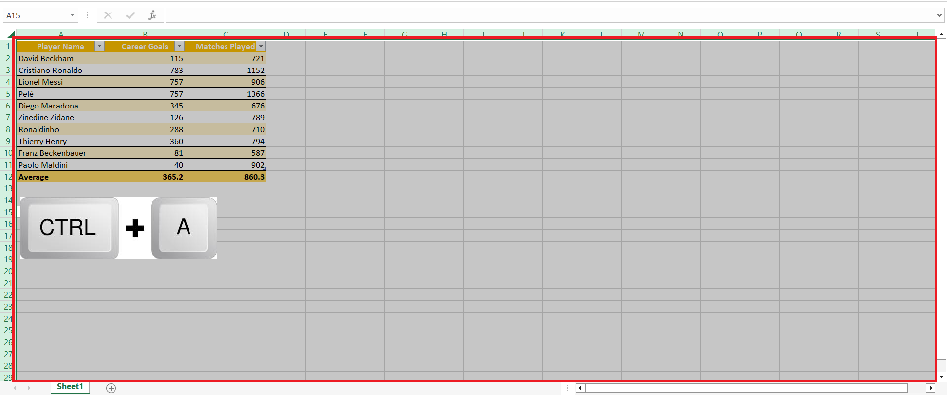
STEP 1: Press Ctrl + A or click the ‘Select All‘ button at the top-left corner of your sheet to highlight everything.

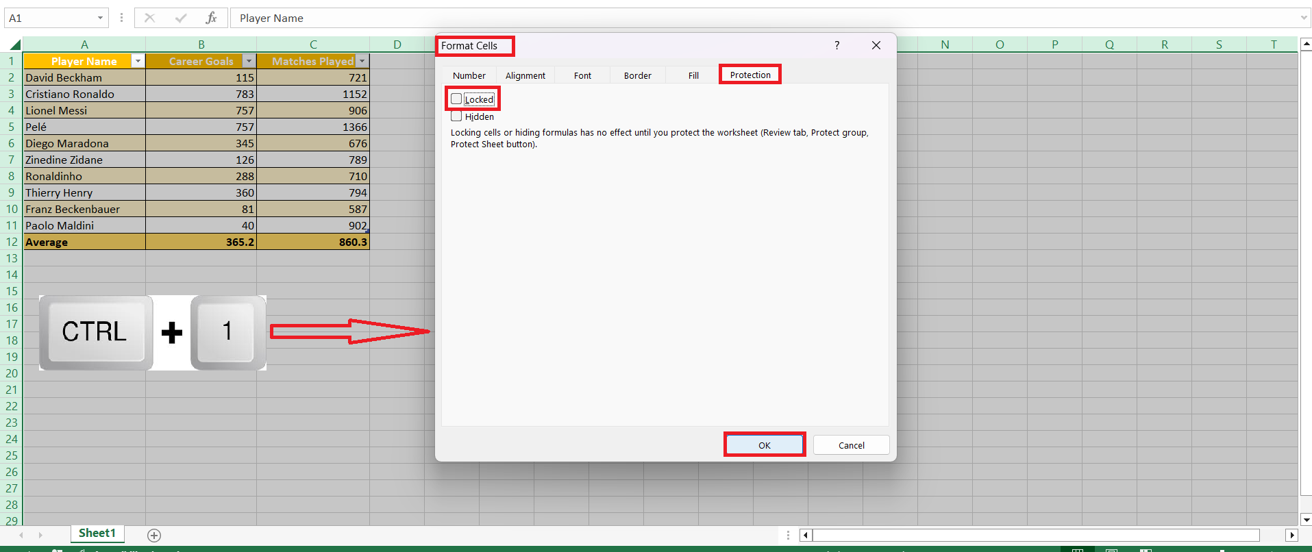
STEP 2: Now, open the Format Cells dialog with Ctrl + 1, head over to the Protection tab, uncheck the ‘Locked’ option, and click ‘OK’. It’s like setting all your guards to “at ease” before you tell them exactly which valuables to defend.

STEP 3: Now that you’ve laid the groundwork, let’s pinpoint the cells that need locking. Navigate back to your earlier selection of cells or ranges that hold the data you want to protect.

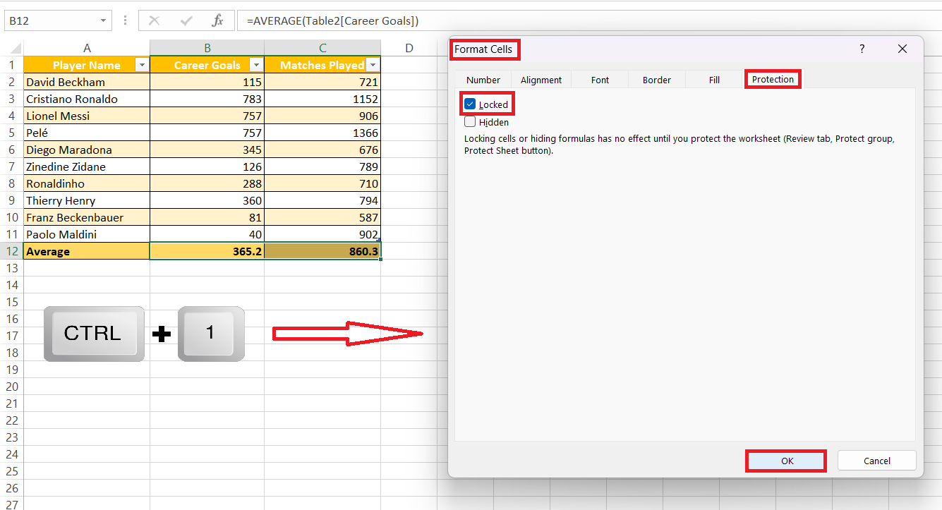
STEP 4: Open up the Format Cells dialog again—there’s a shortcut for this: Ctrl + 1. Under the Protection tab, you’ll see that ‘Locked’ option waiting for you. Check this tag, and you’re essentially telling Excel, “Keep an eye on these!”.

STEP 5: Once you click ‘OK’, these cells aren’t locked down just yet. For the changes to take effect, the final step is to activate sheet protection. But don’t rush there; make sure you’ve accurately marked all the cells on your list first.

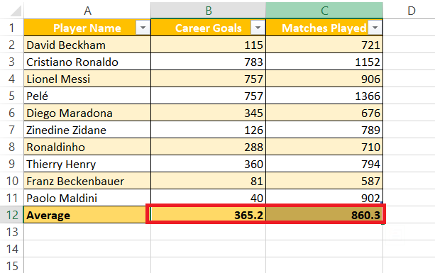
• RESULT:

Advanced Cell Protection Techniques

Locking Formula Cells to Prevent Tampering

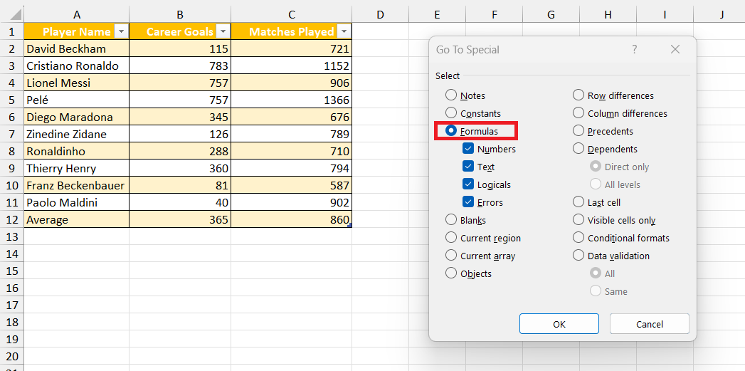
Time to get strategic and shield your formulas from accidental or intentional meddling—locking formula cells is like putting your most important assets in a safe. And the process can be quite straightforward. After ensuring all cells are unlocked as we’ve said earlier, you’ll want to use Excel’s ‘Go To Special’ function by clicking on the ‘Home’ tab, then ‘Find & Select’. Choose ‘Formulas’ and voilà! All cells containing formulas are highlighted.

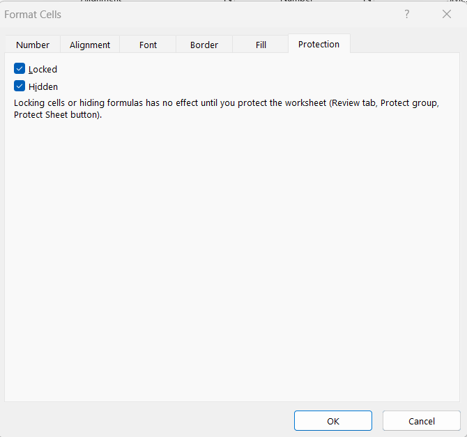
Now, hit Ctrl + 1 to access the ‘Format Cells’ dialog box once more and check the ‘Locked’ box. For an added cloak of invisibility, check the ‘Hidden’ option too, this will keep the formulas concealed in the formula bar.

Once you apply sheet protection, these cells become untouchable to users without the password. And just like that, your formulas are safeguarded.

Customizing Permissions and Locking Certain Cells for Specific Users

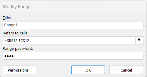
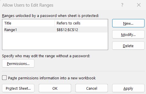
Got a team? Then you’ll love this! You can fine-tune who gets the keys to different parts of your Excel kingdom. Customizing permissions is like assigning different access badges to your crew. Begin by unlocking your worksheet and then hop over to the ‘Review’ tab and click on ‘Allow Users to Edit Ranges’. This powerful feature enables you to set permissions for specific ranges.

Add a New range, input the cells, or use your mouse to make the selection directly on the worksheet, and click ‘Permissions’.

Here, you can add the users who can edit these cells, even after you’ve put the worksheet under protection.

After setting up user names and permissions, confirm and apply your settings, then protect the sheet. Think of it as setting up VIP access; those with clearance can waltz right through, with no password hassle.

 

Protecting Your Entire Worksheet with Special Considerations

How to Keep Your Worksheet Editable While Protecting Data

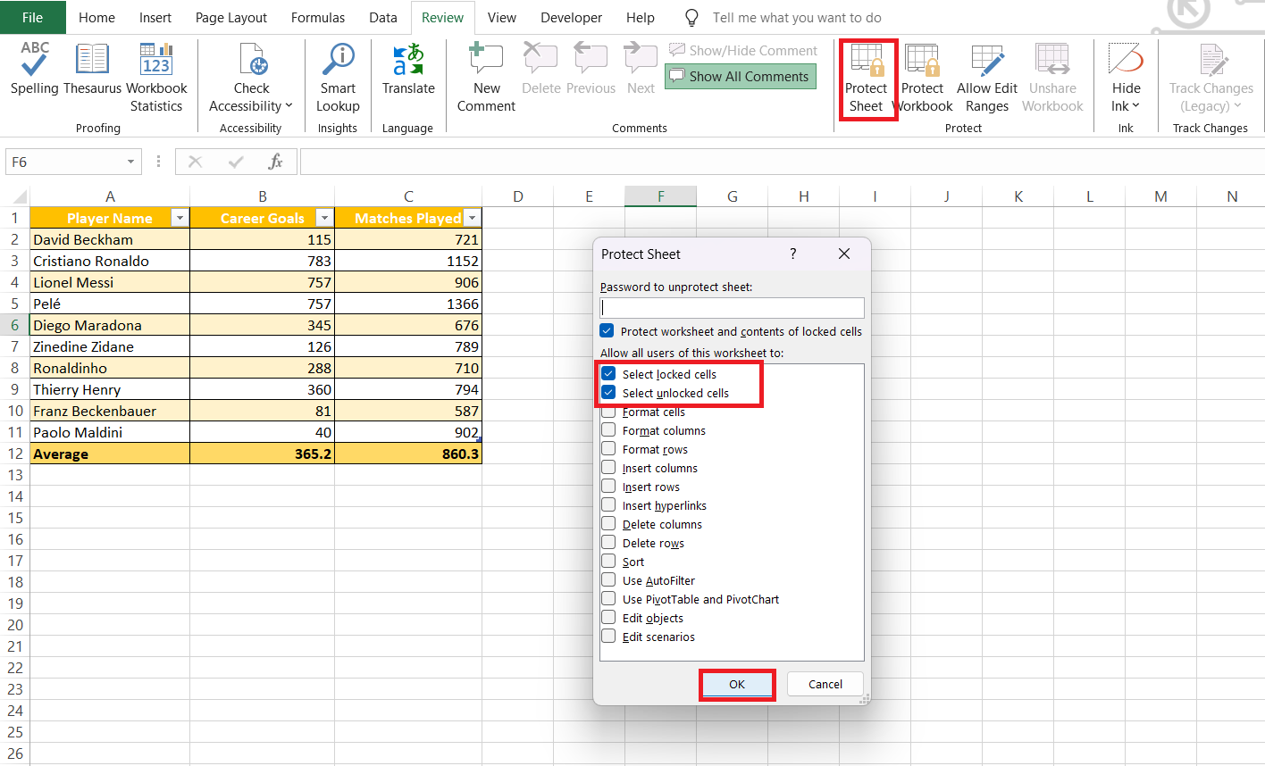
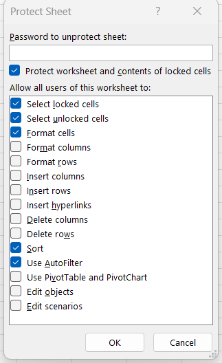
Protect your data without turning your worksheet into a no-go zone. This balancing act is achievable by carefully locking down just your valuable data while keeping the rest of the worksheet open for business. Once you’ve locked your selected cells, head up to the ‘Review’ tab on Excel’s ribbon and click on ‘Protect Sheet’. Here comes the crucial part: in the dialog box that pops up, you’ll see options to allow certain types at of edits—like allowing users to format, sort, or use AutoFilter.

Tick the actions you want to permit, set your password if needed, and hit ‘OK’. Now, you’ve safeguarded your sensitive data, but you’ve also kept the gates open for users to do their work in other parts of the worksheet. It’s like having door guards who know exactly who to let into the party.

 

Tips and Tricks for Excel Users

How to Add Cell Locking Options to the Quick Access Toolbar

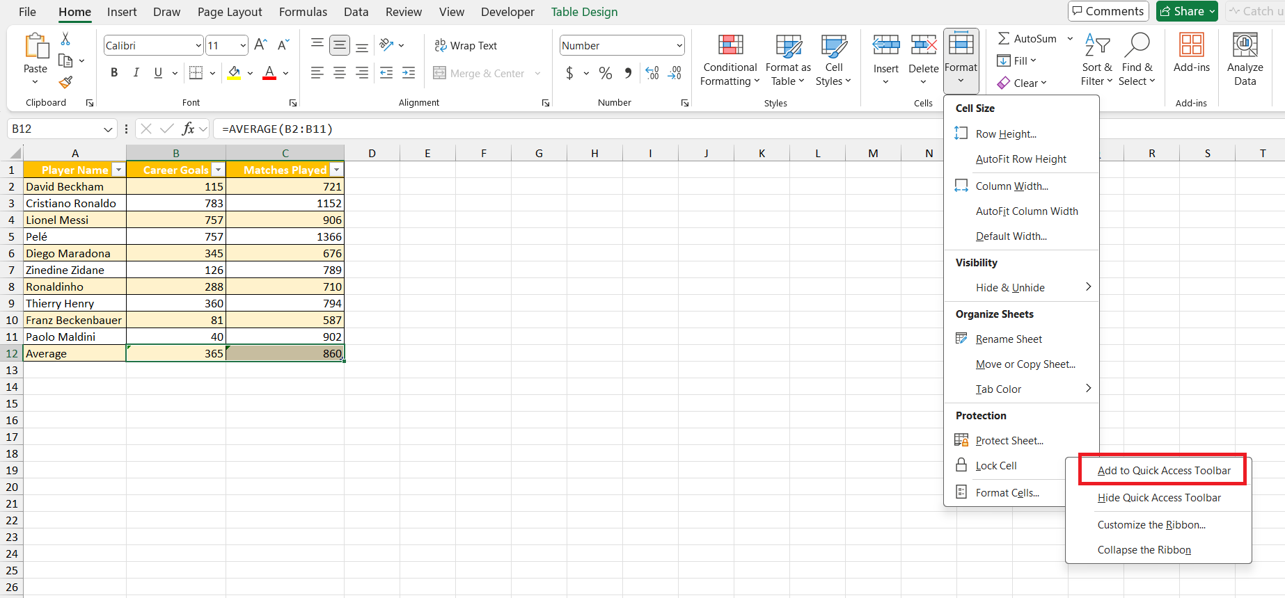
Boost your efficiency by adding the cell locking toggle right to the Quick Access Toolbar (QAT). It’s like having a keychain for your data security measures—you’ll always have the keys handy! Here’s the nifty way to do it: Click on the Home tab and then on the Format button. See that ‘Lock Cell’ option? Right-click on it and select ‘Add to Quick Access Toolbar.

Voilà, it’s now within easy reach for one-click protection. This means less time navigating menus and more time being the Excel wizard you are.

Also, remember, you can customize the QAT to include your most frequently used commands—not just cell locking! Tailor it to your workflow, and watch how smoothly things start to run.

Best Practices for Maintaining Locked Cell Integrity

To keep your locked cells as secure as the Crown Jewels, follow these best practices. Firstly, lock only the cells that need protection—this keeps the sheet functional and user-friendly. Next, always remember to save the workbook immediately after setting your protections to avoid the heartbreak of having to redo it all if something goes awry.

Regularly review your worksheet’s locked cells, especially before distributing the spreadsheet. It’s easy to overlook a cell that ought to be locked, just like a forgotten window in a fortified castle. Additionally, communicate clearly with your team about the protection measures in place. Clarity reduces confusion and preserves the integrity of your data.

 

How to Lock Cells in Excel – FAQs

Can You Sort Data in a Protected Worksheet?

Yes, you can sort data in a protected Excel worksheet – but only if you’ve granted permission for sorting when you set up the sheet protection. To do this, ensure the ‘Sort’ checkbox in the ‘Protect Sheet’ dialog box is selected before applying protection. Remember to unlock any header cells if they’re part of your sorting range!

How Do You Lock Cells Without Protecting the Entire Sheet?

To lock individual cells without protecting the whole sheet, first unlock all cells via Format Cells > Protection tab. Then, select the cells you wish to protect, return to the Format Cells dialog, check ‘Locked’, and then protect the sheet, allowing for certain editing tasks like selecting unlocked cells.

Is It Possible to Lock Cells for Certain Users Without a Password?

Yes, it’s possible to lock cells for certain users without a password by using the ‘Allow Users to Edit Ranges’ feature in Excel. Set up permissions for specific ranges that define which users can edit them, without needing a password for those ranges.

How Can You Identify Whether a Cell Is Locked or Not?

To identify whether a cell is locked or not in Excel, you can use the CELL function. For instance, entering =CELL(“protect”, A1) will return 1 if A1 is locked and 0 if it’s not. This simple function can be extended to check multiple cells at once for quick identification.

What is the shortcut key to choose the protection tab?

The shortcut key to choose the Protection tab directly in Excel is “Ctrl + 1”. This key combination opens the Format Cells dialog box, where you can switch to the Protection tab to access the cell locking features.