Sum the Last 7 Transactions with the Offset Function

In this tutorial, you will learn how to show Excel Sum Last 3 Entries in a Row using the OFFSET function. The OFFSET function in Excel is one of the Lookup functions and is great if you want to reference a range of cells and use that reference to do a calculation. Let’s understand the basics of an OFFSET Function by going through the Formula Breakdown below.

Key Takeaways

• Dynamic Range Creation: The OFFSET function allows you to create a dynamic range by specifying the starting point, number of rows, and columns to include. This is particularly useful when summing the most recent transactions in a dataset.
• Summing Recent Entries: By combining OFFSET with the SUM function, you can calculate the total of the last 7 transactions (or any specific number) without manually updating the range as new data is added.
• Integration with COUNTA: To make the formula more flexible, you can use the COUNTA function to identify the number of non-empty rows in the dataset, ensuring that the OFFSET function targets the correct range.
• Adaptable for Growing Data: This approach adjusts automatically as new rows are added, making it ideal for dynamic datasets where the number of entries changes frequently.
• Customizable Range Length: The formula can be tailored to sum any desired number of recent transactions by simply modifying the row offset parameter, giving you control over the scope of your calculations.

What does it do?

It returns a reference to a range, from a starting point to a specified number of rows, columns, height, and width of cells

Formula breakdown:

=OFFSET(reference, rows, columns, [height], [width])

What it means:

=OFFSET(start in this cell, go up/down a number of rows, go left/right a number of columns, height of range, width of range)

---

Click here to see how the formula works visually & interactively 

Now that you are familiar with the OFFSET function, let’s move ahead and understand how to show Excel Sum Last 7 Entries in a Row.

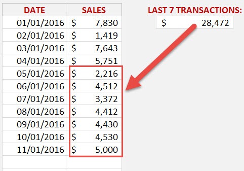
It is often used when you need to reference a range that is moving or resizing. For example, if we have daily sales going down one row per day, then we can Sum the last X transactions.

How to Sum the Last 7 Transactions with the Offset Function

STEP 1: We need to enter the Sum function as we are going to Sum the last 7 transactions

(We can also add the Average function if we want to show the Average of the last 7 transactions):

=SUM

 

STEP 2: We need to enter the Offset function so we can reference the range that we want to Sum:

=SUM(OFFSET

 

STEP 3: 1st Offset argument – Where do we want to to start our reference?

This is at the start of the Daily Sales list:

=SUM(OFFSET(D11

 

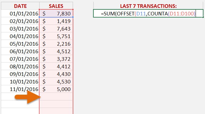
STEP 4: 2nd Offset argument – How many Rows down do we want to go?

This is where the COUNTA function is used to count how many transactions we have in total and go down to the last cell in our list.

So as we are starting at cell D11, we are going to go down 11 cells ( COUNTA(D11:D100) ) and end up after the last cell with a value.

NB: It is always a good idea to enter an ending range that is more than your last data cell.  That way as your new data get entered, we will be sure to capture it!

=SUM(OFFSET(D11, COUNTA(D11:D100)

 

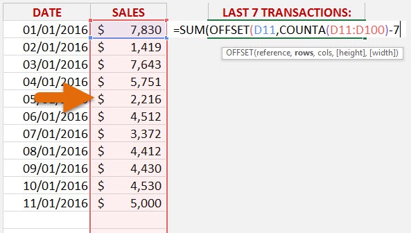
STEP 5: How many of the last sales transactions do we want to Sum?  7

So we need to take away 7 from the COUNTA formula which means that our Offset function will go up by 7 cells:

=SUM(OFFSET(D11, COUNTA(D11:D100)-7,

 

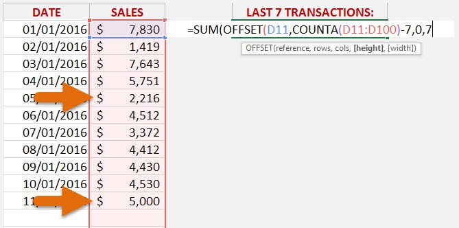
STEP 6: 3rd Offset argument – How many Columns to the right/left do we want to move?

We do not want to move to any Columns, so we simply enter 0

=SUM(OFFSET(D11, COUNTA(D11:D100)-7,0,

 

STEP 7: 4th Offset argument – How High do we want our referenced data to be?

Since we want to Sum 7 transactions, then we need the [height] to be 7 cells high:

=SUM(OFFSET(D11, COUNTA(D11:D100)-7,0,7,

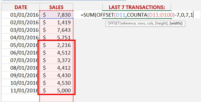
STEP 8: 5th Offset argument – How Wide do we want our referenced data to be?

We want to reference 1 Column only, so we need to enter 1 for the [width]

=SUM(OFFSET(D11, COUNTA(D11:D100)-7,0,7,1))

As we can see the Sum of the last 7 transactions from our example is $28,472.

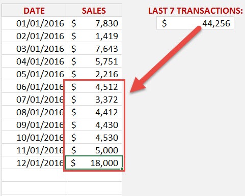
If we add more transactions at the bottom of our Sales list then it automatically returns us the last 7 transactions, without the need to update the formula 🙂

This completes our tutorial on Excel sum last 7 values in row!

Frequently Asked Questions

What is the OFFSET function in Excel, and how does it work?
The OFFSET function in Excel creates a reference to a range based on a starting point, a specified number of rows and columns to offset, and the desired range size. It’s useful for dynamic calculations, such as summing the last 7 transactions, because the referenced range updates automatically as data changes.

How can I use the OFFSET function to sum the last 7 transactions?
To sum the last 7 transactions, use a formula like =SUM(OFFSET(A1, COUNTA(A:A)-7, 0, 7)), where column A contains the transaction amounts. This formula dynamically calculates the sum of the last 7 rows by using the COUNTA function to find the total rows and the OFFSET function to select the last 7.

What happens if my data has less than 7 rows?
If your data has fewer than 7 rows, the formula will throw an error because the OFFSET function cannot reference a range that does not exist. To handle this, use an IF statement or a MAX function, such as =SUM(OFFSET(A1, MAX(0, COUNTA(A:A)-7), 0, MIN(7, COUNTA(A:A)))), to ensure the formula adapts to smaller datasets.

Can I sum a different number of transactions, like the last 10 or 5, instead of 7?
Yes, you can adjust the formula to sum any number of transactions by replacing the -7 and 7 in the OFFSET formula with your desired number, such as -10 and 10 for the last 10 transactions or -5 and 5 for the last 5.

What are the advantages of using OFFSET for summing recent transactions?
Using the OFFSET function provides a dynamic solution that automatically updates as new transactions are added. This eliminates the need for manual adjustments to the range and ensures accuracy in calculations for frequently changing datasets.