UNIQUE Formula in Excel

If you’re someone who frequently works with Excel, you’ve probably encountered the frustration of messy spreadsheets filled with duplicate entries, cluttered lists, and repetitive data. These issues are a common challenge for anyone managing large datasets. I remember spending hours manually filtering or creating pivot tables just to isolate distinct values. That all changed when I discovered the UNIQUE formula—it truly transformed the way I work with data.

In this article, I’ll explain what the UNIQUE function is, why it has become one of my go-to tools, how it operates, and the smart ways it has helped me save significant time—sometimes even entire days. I’ll also highlight common errors, share practical tips, and walk through real-world examples. Whether you’re just starting out with Excel or you’re a seasoned data pro, the UNIQUE formula is a tool you’ll want to keep in your arsenal.

Key Takeaways:

• The UNIQUE function extracts distinct values from a range and updates automatically as data changes.
• You can filter for values that appear only once using the third argument in UNIQUE.
• UNIQUE pairs well with SORT and FILTER to create dynamic, clean, and actionable lists.
• It works both row-wise and column-wise, depending on how your data is structured.
• Common issues like #SPILL! errors or compatibility limitations can be easily resolved with workarounds.

 

Understanding the UNIQUE Function in Excel

What is the UNIQUE Function?

The UNIQUE function is a dynamic array function introduced in Excel 365 and Excel 2019. In simple terms, it extracts unique values from a range or array. Unlike older methods (like using Remove Duplicates or array formulas with IF, COUNTIF, or INDEX/MATCH), this function updates automatically when the source data changes — no more manual refreshing!

Here’s the basic syntax:

=UNIQUE(array, [by_col], [exactly_once])

Let’s break this down:

• array – The range or array from which you want to extract unique values.
• by_col – Optional. Set to TRUE to compare columns instead of rows.
• exactly_once – Optional. Set to TRUE to return only values that appear exactly once.

Why I Use UNIQUE All the Time

Before this function came along, identifying duplicates or extracting distinct values involved a lot of gymnastics — helper columns, sorting, filtering, and mental exhaustion. Now? I just plug in =UNIQUE() and watch Excel work its magic.

Some common scenarios where I use it:

• Listing distinct customer names from sales data.
• Extracting product SKUs for inventory reports.
• Finding all the departments an employee has worked in.
• Cleaning email lists to avoid sending duplicates.

The fact that it’s dynamic — meaning the results auto-update — means I can trust my sheets to stay clean as the data evolves. No more “Oops, forgot to remove that duplicate again.”

 

Practical Applications of the UNIQUE Formula in Excel

Basic Example: Pulling Unique Names

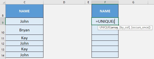
STEP 1: We need to enter the UNIQUE function in a blank cell:

=UNIQUE(

STEP 2: The UNIQUE arguments:

array

What is the data to be cleared of duplicate values?

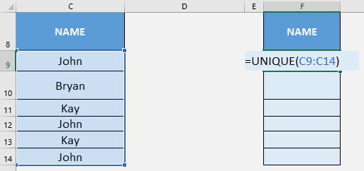
Select the cells containing the names, do not include the headers:

=UNIQUE(C9:C14)

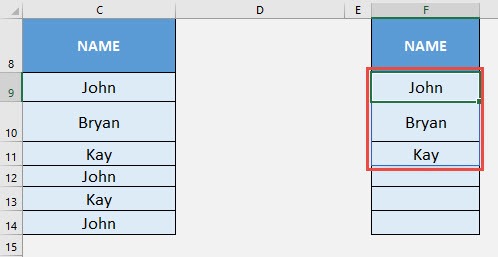
Now the duplicate names are all gone!

Rows vs. Columns

By default, UNIQUE compares rows. But if I’m working with horizontally arranged data, I use the second argument:

=UNIQUE(A1:F1, TRUE)

That tells Excel to compare columns instead of rows. Super handy when I get exported CSVs or pivoted data where the values are laid out sideways.

Advanced Usage of Unique Formula

Extract Unique Data Appearing Exactly Once

Let’s say I’m only interested in values that appear exactly once — no repeats at all. This is where the third argument becomes powerful:

=UNIQUE(A2:A20,,TRUE)

This will only return values that show up once in that list. I use this often when auditing customer complaints or support tickets — I only want to see the one-off cases.

Combining UNIQUE with SORT and FILTER

In Excel, the UNIQUE function pairs exceptionally well with the SORT function to create organized and efficient data outputs. One commonly used combination is:

=SORT(UNIQUE(A2:A8))

This formula generates a sorted list of unique entries from the specified range, making it particularly useful for creating dropdown menus, dashboards, and summary reports.

Additionally, when combined with the FILTER function, the UNIQUE function becomes even more powerful. For example:

=UNIQUE(FILTER(A2:A8, B2:B8=”Completed”))

This formula returns only the distinct values from column A where the corresponding status in column B is marked as “Completed.” It is especially effective for generating dynamic lists such as completed projects, fulfilled orders, or confirmed attendees.

When UNIQUE Doesn’t Work (and How I Fix It)

Even magic functions have their quirks. Here are a few issues I’ve run into:

1. #SPILL! Error

UNIQUE is a dynamic array function, so it “spills” its results into multiple cells. If those cells aren’t empty, you’ll get a #SPILL! error.

Fix: Clear the space below your UNIQUE formula so it can spill freely.

2. UNIQUE Doesn’t Exist

This function only works in Excel 365 and Excel 2019+. If you’re using an older version, you won’t find it.

Workaround: Use Advanced Filter or pivot tables for similar behavior, but it’s nowhere near as smooth.

3. Blank Cells in the Output

If your original data has blank cells, UNIQUE will include them. To remove blanks, nest it inside a FILTER:

=UNIQUE(FILTER(A2:A100, A2:A100<>””))

FAQs

1. What does the UNIQUE function do in Excel?

The UNIQUE function returns a list of unique values from a selected range or array. It’s part of Excel’s dynamic array functions, which means the output automatically adjusts when source data changes. This makes it especially useful for maintaining clean, duplicate-free datasets without manual filtering. It’s more efficient than traditional methods like using pivot tables or helper columns.

2. How do I extract values that appear only once?

To return only values that occur exactly once in a range, you can use the third argument of the UNIQUE function. For example:

=UNIQUE(A2:A20,,TRUE)

This filters the range to include only one-time entries, which is useful when analyzing anomalies, one-off records, or cases that shouldn’t repeat — such as unique customer complaints or single-instance transactions.

3. Can I use UNIQUE on horizontal (row-based) data?

Yes, you can. By default, UNIQUE compares values vertically (by rows). However, if your data is structured horizontally across columns, you can set the second argument to TRUE. For example:

=UNIQUE(A1:F1, TRUE)

This compares columns instead of rows, which is useful when dealing with transposed or pivoted data.

4. What’s the benefit of combining UNIQUE with SORT and FILTER?

Combining these functions allows you to create highly dynamic and user-friendly outputs. For instance, SORT(UNIQUE(range)) provides an alphabetically sorted list of distinct entries, ideal for dropdowns and reports. Adding FILTER lets you extract condition-based unique entries — like only showing completed projects or approved submissions — making your data output cleaner and context-specific.

5. What do I do if UNIQUE gives a #SPILL! error or doesn’t work?

The #SPILL! error usually means there’s not enough space for the dynamic array to output its results. Clear the cells below or beside the formula to fix it. If the function doesn’t exist at all, you’re likely using an older Excel version (pre-2019 or Office 365). In that case, you can use pivot tables or Advanced Filters as a workaround, though those methods are static and require manual updates.