How to Abbreviate Numbers in Excel – Step by Step Guide

Working with large numbers in Microsoft Excel can sometimes feel challenging, especially when you’re creating reports or dashboards. If you’ve ever wished to replace those long numbers with something more concise like “1K” or “1M,” you’re not alone. In this article, I’ll show you step-by-step how I abbreviate numbers in Excel to make my spreadsheets look cleaner and easier to read.

Key Takeaways:

• Abbreviating large numbers in Excel makes spreadsheets cleaner and more readable.
• Custom number formatting in Excel lets you display numbers in concise forms.
• Formulas like IF and TEXT can provide flexibilty and text based abbreviation.
• Custom Format can improve precision in calculations.
• Consistent decimal formatting provides a professional, uniform spreadsheet.

Abbreviate Number: Key Excel Tricks

Method 1: Create a Custom Format Code

Follow the steps below to create a custom code in Excel:

STEP 1: Select the cell or range of cells that require formatting.

STEP 2: Go to the Home tab and select More Number Formats from the dropdown.

STEP 3: In the Number tab, select Custom.

STEP 4: Type a custom format. For example:

Use #,, “Million” to convert 1000,000 into 1 Million.

This custom format will be saved in the worksheet and can be used later as well.

However, when we are working on a new workbook, we will have to copy the custom format into it.

Method 2: Use Formulas

You can use a combination of IF and TEXT to create a formula to abbreviate a number:

Explanation:

• A2>=1000000000: Checks if the number is greater than billions.
• TEXT(A2/1000000000, “0.0”) & “B”: Converts billions into abbreviated text like #.#B
• A2>=1000000: Checks if the number is greater than millions.
• TEXT(A2/1000000, “0.0”) & “M”: Converts millions into abbreviated text like #.#M
• A2>=1000: Checks if the number is greater than 1000.
• TEXT(A2/1000, “0.0”) & “K”: Converts thousands into abbreviated text like #.#K
• If all these conditions are false, then the original number will be displayed.

Method 3: Using Conditional Formatting

You can use Conditional Formatting to abbreviate the number and keep the underlying value the same. Follow the steps below:

Select the range and go to Home > Conditional Formatting > New Rule.

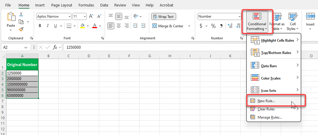
Select Use a formula to determine which cells to format.

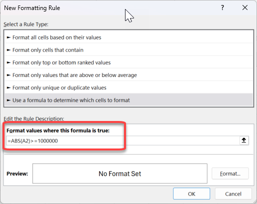
Use formulas like:

• =ABS(A1)>=1000000 → Apply formatting with an “M” suffix.
• =ABS(A1)>=1000000000 → Apply formatting with a “B” suffix.

Make sure to apply the formulas in the correct order, and your result will look like this:

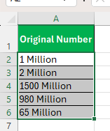
This method keeps the numeric value intact for calculation and only changes the display.

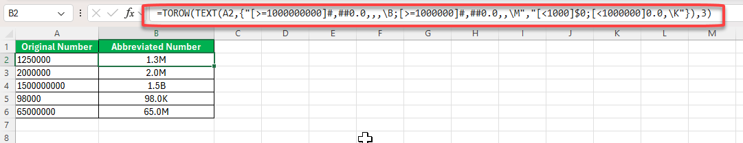
Method 4: TOROW function

You can use the combination of dynamic arrays and the TOROW function to abbreviate numbers in Excel.

 

Tips & Tricks

Add Suffix

You can abbreviate long numbers into a quick, readable format by using suffixes like K or M. Follow the steps below to add these suffixes:

• Right-click on the cell
• Select Format Cells.
• Under the Number tab, select Custom
• Type #,##0,"K";(#,##0,"K") for thousands.

Type #,##0,,"M";(#,##0,,"M") for millions.

This format will abbreviate numbers and show negative numbers within parentheses.

Truncating Numbers

Truncating a number is useful when you want to make the numbers look clean, but not change the underlying value. You can achieve this by using a custom format in Excel.

For example: Use format #,”K” to change 117943 to 118K

This format can be used when creating dahsboard sor reports to display numbers in a clean format. The number will maintain its integrity, and the results are precise.

 

FAQ Section

How to Automatically Abbreviate Numbers in Excel?

To have Excel automatically abbreviate numbers, create a custom number format. Under ‘Format Cells‘, choose ‘Custom’ and enter a format code using placeholders and symbols. For example, “0,” will display thousands as ‘K’, and “0,,” for millions as ‘M’ without changing the actual number’s value. Apply this to the relevant cells, and Excel will abbreviate the numbers as you type them in.

Why Are My Abbreviated Numbers Not Showing Correctly in Excel?

Consider the following points when the abbreviated numbers are not displayed correctly:

• Double-check for any typing errors or incorrect symbols in the format string.
• Check that the actual value corresponds to the format. For example, K will not be displayed if the value is less than 1000.
• Check that the language and regional number format setting is correct.

How to abbreviate thousands and millions in Excel?

You can abbreviate thousands and millions by following the steps below:

• Right-click on the cell that you want to format.
• Select Format Cells.
• In the Number tab, select Custom.
• Type #,##0,”K” for thousands, #,##0,,”M” for millions.
• Click OK.