The Ultimate Guide to Excel Data Table Analysis

Excel is a powerful tool in data analysis, serving as a cornerstone for users across numerous professions. Among its myriad of functionalities, data tables are paramount in simplifying complex numerical data analyses. This guide will take you through the detailed process of leveraging Excel data tables to enhance your analytical capabilities, optimize performance, and provide insights that drive informed decisions.

Key Takeaways:

• Excel Data Tables are part of the What-If Analysis tools for scenario planning.
• One-Variable Data Table changes one input and shows multiple results instantly.
• Two-Variable Data Table helps analyze the impact of changing two inputs together.
• Data Tables save time and avoid manual recalculations for multiple scenarios.
• They are widely used in financial modeling, budgeting, and forecasting tasks.

 

Understanding Excel Data Tables

What are Data Tables?

Data tables in Excel are part of the What-If Analysis tools, designed to showcase how variations in input values impact the output of a formula. Unlike a regular Excel table, which manages related data, data tables offer a dynamic view of potential outcomes by facilitating the analysis of variable combinations.

There are two main types of data tables: one-variable tables, which allow the analysis of a single variable, and two-variable tables, which offer insights when modulating two different inputs. This functionality is especially potent for financial modeling, forecasting, and sensitivity analysis, providing a visual and comparative overview of other scenarios.

The Importance of Using Data Tables

Data tables are essential in Excel for several reasons, primarily due to their ability to streamline and simplify the process of scenario analysis. By allowing users to alter one or two variables and instantly observe the effect on outcomes, data tables save time and reduce errors compared to manual recalculation.

This becomes particularly valuable in financial modeling, where they provide quick insights into how assumptions might alter performance metrics. Furthermore, data tables enhance decision-making by presenting a clear visualization of potential results, thereby allowing users to evaluate risks and opportunities with greater precision.

In industries that rely heavily on forecasts and trend analysis, such as finance and operations, this capability significantly supports strategic planning.

 

One-Variable Data Table

What is it?

A One-Variable Data Table is a special feature in Excel that allows me to analyze the impact of changing a single input value in a formula while keeping all other values constant. It helps me observe how the result will vary when only one factor changes.

This feature is useful because it eliminates the need to change the input value manually multiple times and check the output separately. Excel automatically calculates and displays all possible results based on different values of that single variable in a neat and organized table. This makes my analysis faster, easier, and more professional.

I used the One-Variable Data Table in one of my loan calculation projects. I had to calculate the EMI for a loan amount of $500,000 with a repayment period of 5 years. The loan amount and the time period were fixed, but the interest rate was uncertain as it kept fluctuating in the market.

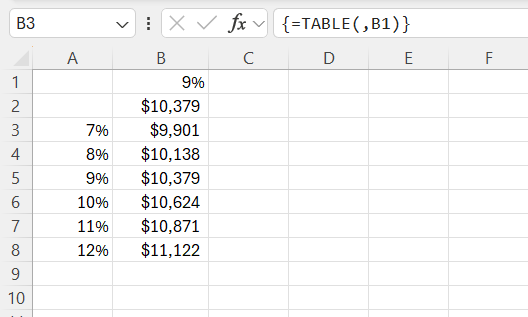
To understand how the EMI would vary with different interest rates, I decided to prepare a scenario where the interest rate changes from 7% to 12%. Using the One-Variable Data Table, I was able to generate all possible EMI values for these interest rates in a single view without changing the formula manually each time.

This helped me analyze and compare the EMI for each interest rate easily and efficiently.

Creating a One-Variable Data Table

Creating a one-variable data table involves a straightforward process that allows you to assess how changes in a single variable affect one or more formulas. Here’s a concise guide to constructing your first one-variable data table efficiently:

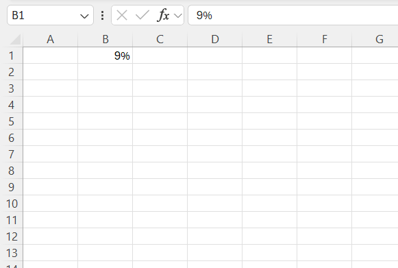
STEP 1: In cell B1, enter the base interest rate (for example, 9%) — this is the cell your formula will refer to for calculations.

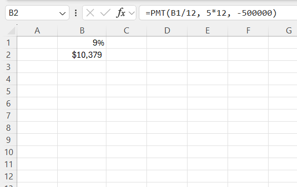
STEP 2: In cell B2, write the EMI formula using the PMT function like this:

=PMT(B1/12, 5*12, -500000)

This formula calculates EMI based on the interest rate in cell B1.

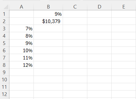
STEP 3: In column A (from A3 to A8), enter different interest rates you want to analyze — for example: 7%, 8%, 9%, 10%, 11%, 12%.

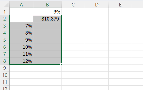
STEP 4: Select the range from A2 to B8 — this includes your interest rate values and the formula output column.

STEP 5: Go to the Data tab → Click What-If Analysis → Select Data Table.

STEP 6: In the Data Table dialog box, since your variable values (interest rates) are in a column, enter B1 in the Column input cell box (because the formula depends on B1 for interest rate).

Click OK.

Excel will instantly calculate the EMI for each interest rate and display the results in column B.

The one-variable data table you’ve created can now offer a visual exploration of how adjusting one factor, like an interest rate, influences the results. This tool is incredibly useful for exploring various scenarios and their potential impacts quickly and accurately.

 

Diving into Two-Variable Data Tables

What is it?

A Two-Variable Data Table is another powerful feature in Excel that allows me to analyze the impact of changing two input values in a formula at the same time while keeping all other values constant. It helps me observe how the result will vary when two factors are changing together.

This feature is highly useful when I want to compare multiple scenarios involving two different variables. Instead of creating multiple formulas manually for every combination, Excel automatically calculates and displays the result for all possible combinations of the two variables in a structured table. This saves time and makes my analysis highly efficient and professional.

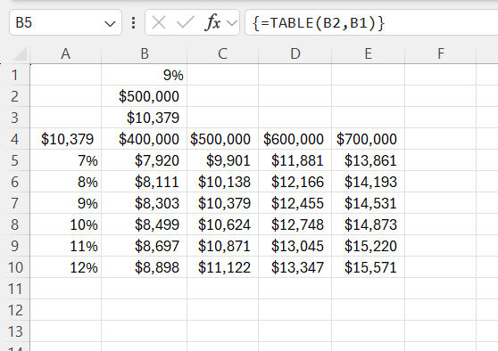
I used the Two-Variable Data Table in the same loan EMI calculation project where I had a loan amount of $500,000 with a repayment period of 5 years. Along with the changing interest rate, I also wanted to see how the EMI would vary if the loan amount also changes.

To do this, I created a Two-Variable Data Table where:

• Interest Rates were changing from 7% to 12% vertically
• Loan Amounts were changing from $400,000 to $700,000 horizontally

Using the Two-Variable Data Table, I was able to generate EMI values for all combinations of interest rates and loan amounts in a single view without changing the formula manually for each case. This helped me analyze and compare the EMI for every scenario very easily.

Creating a Two-Variable Data Table

Creating a two-variable data table allows you to assess how changes in two different variables affect the result of a formula. Here’s a simple step-by-step guide that I follow to create it:

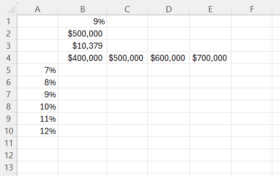
STEP 1: In cell B1, enter the base interest rate (for example, 9%).

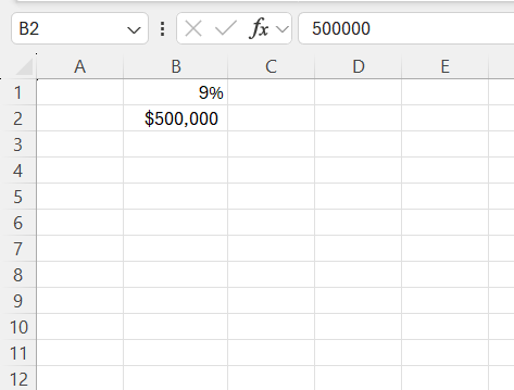
STEP 2: In cell B2, enter the base loan amount (for example, $500,000).

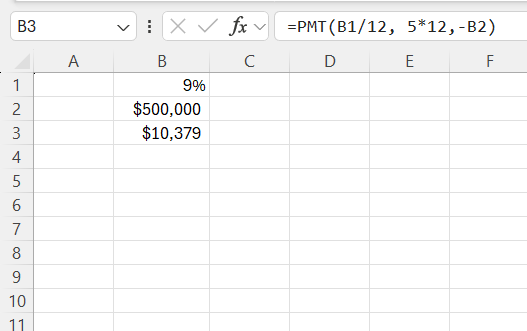
STEP 3: In cell B3, write the EMI formula using the PMT function like this:

=PMT(B1/12, 5*12, -B2)

This formula calculates EMI based on the interest rate in cell B1 and the loan amount in cell B2.

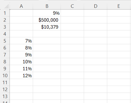
STEP 4: In column A (from A5 to A10), enter different interest rates you want to analyze — for example: 7%, 8%, 9%, 10%, 11%, 12%.

STEP 5: In row 4 (from B4 to E4), enter different loan amounts you want to analyze — for example: $400,000, $500,000, $600,000, $700,000.

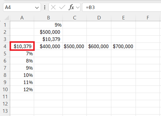
STEP 6: In cell A4 (top-left of your table), link your formula by writing: =B3.

This will display the EMI results once the Data Table is created.

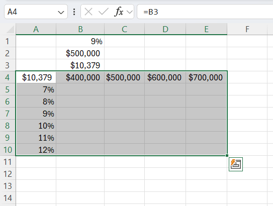
STEP 7: Select the range from A4 to E10 — this includes the interest rate values, loan amount values, and the result area.

STEP 8: Go to the Data tab → Click What-If Analysis → Select Data Table.

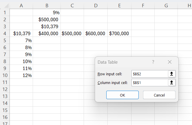
STEP 9: In the Data Table dialog box:

• In Row input cell, enter B2 (because loan amounts are in the row).
• In Column input cell, enter B1 (because interest rates are in the column).

Click OK.

Excel will instantly calculate EMI for each combination of interest rate and loan amount and display the results in the table.

The Two-Variable Data Table is a powerful tool for creating detailed scenario analysis when two factors are involved. It helps me compare results across multiple combinations and makes my financial analysis faster, dynamic, and more insightful.

 

Applications and Use Cases

Two-variable data tables in Excel are immensely valuable across various domains, especially in scenarios where understanding the interplay between different variables is crucial. Here are some key applications and use cases:

• Financial Forecasting: Businesses can utilize two-variable data tables to forecast future cash flows or profits by varying assumptions such as sales volumes and pricing strategies. This helps in crafting more resilient financial plans by anticipating how different conditions might affect the bottom line.
• Budgeting: In budgeting, companies often need to account for changes in expenditure and revenue sources. A two-variable data table can simulate different expenditure levels against various income scenarios, aiding in identifying potential financial shortfalls or surpluses.
• Sales Strategy Planning: Sales teams can analyze the impact of different pricing strategies and customer acquisition rates on revenue. By testing combinations of these variables, they can optimize strategies for meeting sales targets.
• Investment Analysis: Investors can benefit from exploring potential returns under various scenarios by altering inputs like interest rates and investment durations. This helps in assessing the risk and reward profile of different investment options.
• Operational Efficiency: Operations managers can evaluate how changes in labor costs and production volumes might impact overall operating costs. This is useful for optimizing resource allocation and streamlining production processes.

These applications illustrate the adaptability and power of two-variable data tables in delivering actionable insights. By enabling a multifaceted analysis of varying conditions, these tables support informed decision-making across industries, ensuring strategic objectives are achievable under different potential scenarios.

 

Common Mistakes to Avoid

When working with two-variable data tables in Excel, several common mistakes can hinder your analysis. Recognizing and avoiding these pitfalls ensures your data tables function correctly and deliver accurate insights.

• Incorrect Formula Placement: Always ensure that the formula to be analyzed is at the intersection of the row and column headings for the variables. Incorrect placement can lead to faulty or no results.
• Input Cell Reference Errors: Failing to correctly reference the row and column input cells related to the variables can result in inaccurate calculations. Double-check that each input cell corresponds to the correct variable used in your formula.
• Range Selection Oversights: Ensure the entire matrix of the data table, including the formula cell, is properly selected before using the Data Table function. Missing any part of this range can lead to incomplete data.
• Non-consistent Data Type: Using inconsistent data types or units within your variables list can cause Excel to produce errors. Always verify that the variables hold values in the same format or unit.
• Circular Reference Problems: Avoid using formulas in data tables that create circular references, as they can disrupt Excel’s calculation scripts, leading to incorrect outcomes or infinite loops.

By steering clear of these common errors, you can ensure that your two-variable data tables are accurate and useful for analysis. These mistakes often lead to results that can misinform decisions, so it’s important to be meticulous during setup to maintain data integrity and analytical reliability.

 

FAQs

What is data table analysis in Excel?

Data table analysis in Excel is a powerful What-If Analysis tool that allows users to observe how changes in input variables affect the outcomes of formulas. It provides a dynamic way to explore multiple scenarios by adjusting one or two key inputs and visualizing the results, facilitating better decision-making and strategic planning.

How do I manually recalculate a data table?

To manually recalculate a data table in Excel, first select the entire range of the table output cells, which contain the TABLE() formulas. Then, press the F9 key. This action will trigger the recalculation of the specified data table, updating its results based on the current input values.

Can I use formulas within data tables?

Yes, you can use formulas within data tables. The data table utilizes a formula to generate results based on changing input variables. However, it’s important that the formula in the intersection cell references the input variables properly so that the data table can dynamically update the outcomes as you vary these inputs.

What are the limitations of Excel data tables?

Excel data tables have several limitations: they can only work with one or two input variables, making them less suitable for complex models with more variables. They also require all data to be on the same worksheet and can slow performance in large files. Additionally, data tables cannot integrate with other Excel features, such as PivotTables or external data sources.

Do Data Tables automatically update if input values change?

Yes, Data Tables in Excel update automatically when input cells change. However, if you have manual calculation mode on, you may need to press F9 to refresh the table values.