Filter by Values – Top or Bottom Sum

Pivot Table allows you to filter by values that make the top or bottom based on a specific sum. For example, you get the top records that account for 1,000,000 of the total sales. Let us see this in action!

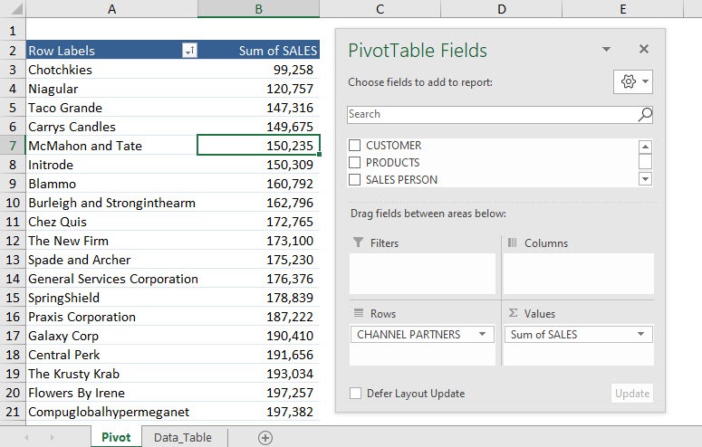
This is our current Pivot Table setup. We will be filtering the Top Channel Partners that account for 1,000,000 of total sales.

 

Example 1: Filter by Values – Top

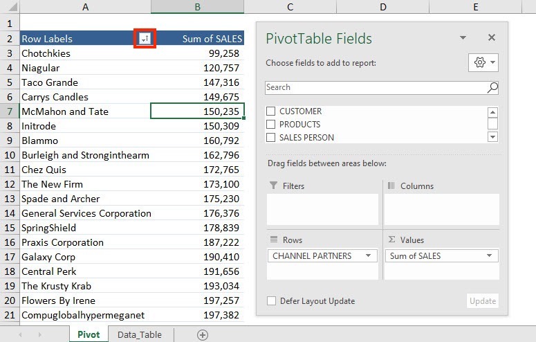
STEP 1: Click on the Row Label filter button in the Pivot Table.

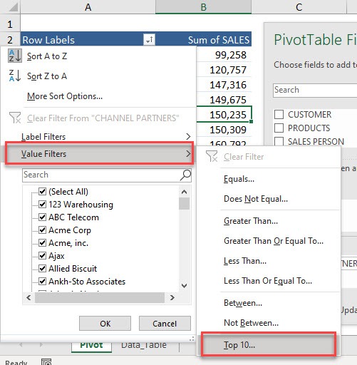
STEP 2: Select Value Filters.

You will see that we have a lot of filtering options. Let us try out – Top 10

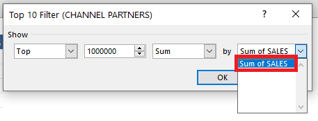
STEP 3: Since, you want the list of Top channel partners that makes 1,000,000 of total sales – select the Top in the first field.

STEP 4: In the second field, mention the value that the top channel partners should account for – type 1000000.

STEP 5: In the third field, select Sum.

STEP 6: The fourth field, lists all the values mentioned in the values area of the Pivot Table.

Select sum of values.

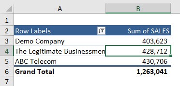
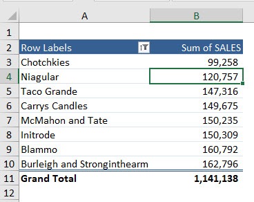
Now you have the top channel partners that when combined, will give you at least 1,000,000 for the sum of sales.

 

Example 2: Filter by Values – Bottom

STEP 1: Click on the Row Label filter button in the Pivot Table.

STEP 2: Select Value Filters and Top 10.

STEP 3: Select the Bottom in the first field, 1,000,000 in the second field, and Sum in the third field.

Select Sum of SALES in the fourth field and click OK.

Now you have the bottom channel partners that when combined, will give you at least 1,000,000 for the sum of sales.

Following the steps mentioned above, you can easily filter the Pivot Table by values and list the Top or Bottom items based on the sum of values. You can also use Pivot Table to filter Top/Bottom items by Percentage, filter items based on Value, etc.

Frequently Asked Questions

How do I filter for top 10 values in a Pivot Table?
Click the filter drop-down on the field, choose Value Filters > Top 10, then set the number, type (Items, Percent, Sum), and target field.

Can I filter by bottom values instead of top?
Yes, choose Bottom instead of Top in the Value Filter dialog box to display the lowest-ranking items.

What’s the difference between filtering by top items and top sum?
Top items shows a set number of entries, while top sum includes entries that collectively reach a specified total or percentage.

Can I apply top/bottom filters outside Pivot Tables?
Yes, use the Number Filters > Top 10 option on a regular table column to apply a similar filter.

Will my top/bottom filter update automatically with new data?
Yes, if you’re using a Pivot Table or Excel Table, the filter adjusts when data is refreshed or updated.