Scrolling through large Excel sheets can be frustrating when your headers disappear off screen. To improve readability and keep your important context visible, you can freeze rows at the top. In many reports, it’s not just the first row that needs freezing. Sometimes, you have two header rows that should stay visible while navigating. In this guide, you’ll learn how to freeze top 2 rows in Excel using a simple and reliable method.
Key Takeaways
- Use Freeze Panes to lock specific rows or columns in place
- To freeze top 2 rows, select row 3 before using Freeze Panes
- This method works the same in Excel for Windows and Mac
- Freezing rows helps maintain header visibility while scrolling
- You can unfreeze anytime by choosing Unfreeze Panes
Table of Contents
Why Freeze Rows in Excel?
Freezing rows ensures that key information like headers or labels stay visible when scrolling down through large datasets. If your worksheet includes two rows of column headings or categories, freezing both helps keep that structure intact. Excel allows you to freeze any number of rows from the top, but you must follow specific steps to do it correctly.
Understanding the Basics of Freeze Panes
Freeze Panes is a handy Excel feature that lets you lock specific rows or columns in place, allowing them to stay visible as you scroll. This is particularly useful in datasets with multiple entries, helping you keep headers or important data always within view. To freeze the top two rows, navigate to the “View” tab, select “Freeze Panes,” and choose “Freeze Top Row” twice or select “Freeze Panes” and then unfreeze to customize further.
Key Benefits of Freezing Rows in Excel
Freezing rows in Excel offers several benefits that enhance data management efficiency. Firstly, it ensures important headers or labels remain visible, allowing for easy referencing as you scroll through large datasets. This visibility can prevent data entry errors and streamline data analysis. Secondly, it can simplify navigation across extensive spreadsheets, aiding in quick access to key information. Additionally, it enables a more organized presentation, especially while demonstrating data in meetings or collaborative settings.
How to Freeze Top 2 Rows in Excel
Step 1: Set Up Your Data
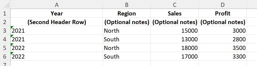
Start with a sheet that has at least two rows you want to keep visible. For example:
Step 2: Select the Row Below the Ones You Want to Freeze
To freeze the top 2 rows:
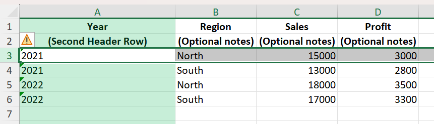
Click on row number 3 in the worksheet
This highlights the entire third row
Step 3: Apply Freeze Panes
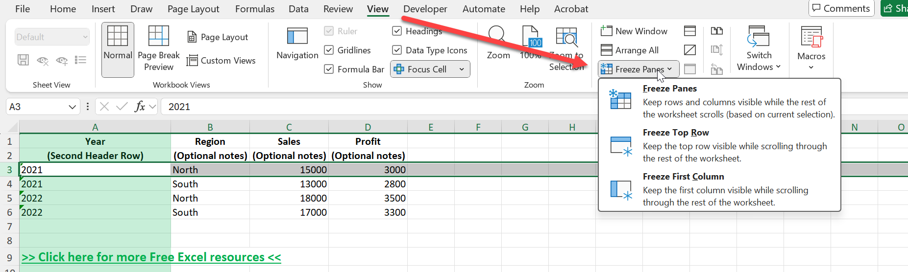
With row 3 selected:
Go to the View tab on the Ribbon
Click the dropdown for Freeze Panes
Select Freeze Panes (not Freeze Top Row)
Excel will now freeze everything above the selected row — in this case, rows 1 and 2.
Step 4: Test the Freeze
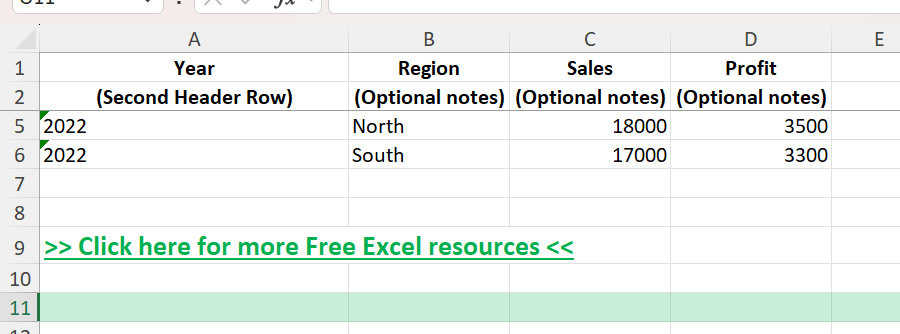
Scroll down the sheet. You’ll notice that rows 1 and 2 remain locked at the top of the screen while the rest of the sheet scrolls beneath them.
Common Mistakes or Tips
Selecting the wrong row: To freeze the top 2 rows, you must select row 3, not the first or second row
Using Freeze Top Row by mistake: That only freezes row 1. To freeze more than one row, always use the general Freeze Panes option
Worksheet already frozen: If nothing happens, go back to Freeze Panes and choose Unfreeze Panes first, then repeat the steps
Hidden rows: If rows 1 or 2 are hidden, unhide them before trying to freeze
Row selection must be entire row: Make sure you click on the row number at the left, not just a cell in the row
Bonus Tips and Advanced Scenarios
Freeze Rows and Columns Together: Select cell C3 to freeze top 2 rows and left 2 columns at the same time
Use Split View for Comparison: If freezing is not flexible enough, try using the Split option under the View tab for more control
VBA to Freeze Rows: You can use a macro to automate freezing if setting up multiple sheets. Example VBA:
Sub FreezeTopTwoRows()
    Rows("3:3").Select
    ActiveWindow.FreezePanes = True
End Sub
Keyboard Shortcuts for Quick Access
Excel offers a variety of keyboard shortcuts to facilitate quick access to frequent actions, including freezing panes. By familiarizing yourself with these shortcuts, you can streamline your workflow significantly. To freeze the first two rows, you might use ALT + W, then F, and select from the options like Freeze Panes, after unfreezing if needed.
These shortcuts improve efficiency by reducing the need to navigate menus with a mouse, making them especially beneficial during data-intensive tasks. Getting accustomed to these shortcuts can also accelerate your data management practices, providing you with more time to focus on analysis rather than navigation. Consider compiling a list of often-used shortcuts and keeping them handy to enhance your productivity further.
Combining Freeze Panes with Other Features
Combining the Freeze Panes feature with other Excel functionalities can significantly enhance your data handling capabilities. For instance, Freeze Panes can be coupled with Conditional Formatting to highlight key data, while maintaining view of vital row information at all times. This creates a more dynamic and informative spreadsheet environment, ideal for thorough data analysis.
Another way to boost efficiency is by using Freeze Panes alongside Filters. By keeping specific information in view, users can more easily apply and modify filters without losing sight of headers or critical data points. Pivot Tables also work well with Freeze Panes, allowing a constant context of table modifications and interpretations being made.
Such combinations provide a powerful toolkit for complex data manipulation, making it easier to draw insights and perform actions based on the most relevant data. While these combined approaches can enhance productivity, ensure to manage the view layout carefully to avoid clutter and maintain a clear focus on your objectives.
Frequently Asked Questions
How do I freeze the top 2 rows in Excel?
Select row 3, go to View > Freeze Panes > Freeze Panes. This locks rows 1 and 2.
Why does Freeze Top Row not work for 2 rows?
Freeze Top Row only freezes row 1. To freeze more than one row, use the standard Freeze Panes option instead.
Can I freeze both rows and columns?
Yes. Select the cell below the rows and to the right of the columns you want to freeze. For example, to freeze top 2 rows and first 2 columns, select cell C3.
How do I remove freezing?
Go to View > Freeze Panes > Unfreeze Panes to remove all freezing on the current sheet.
Can I freeze rows in Excel Online?
Yes, Excel Online supports freezing, but you must use the View tab and select the Freeze Panes option just like the desktop version.

John Michaloudis is a former accountant and finance analyst at General Electric, a Microsoft MVP since 2020, an Amazon #1 bestselling author of 4 Microsoft Excel books and teacher of Microsoft Excel & Office over at his flagship MyExcelOnline Academy Online Course.


