How to Create a Hyperbolic Curve in Excel – Step by Step Guide

Excel makes it easy to chart linear or exponential trends, but what if your data follows an inverse pattern? That’s where hyperbolic curves come in. Whether you’re analyzing cost efficiency, physical systems, or inverse demand, understanding how to model a hyperbolic relationship using Excel formulas and charts can be extremely useful.

This step-by-step guide will walk you through the process of creating a hyperbolic curve in Excel. You’ll learn the formula, build a dynamic chart, and even explore advanced enhancements using VBA and Power Query. A downloadable Excel file is also included so you can follow along and test each step.

Key Takeaways

• Hyperbolic curves represent inverse relationships and follow the formula y = a / x

• Excel handles hyperbolic formulas using standard arithmetic operations

• A scatter plot with smooth lines is the best chart for visualizing hyperbolic data

• Helper cells can make your model dynamic and reusable

• Bonus techniques like VBA scripting and Power Query allow for automation and interactivity

Understanding Hyperbolic Curves in Excel

Basics of Hyperbolic Functions

Hyperbolic functions are mathematical functions that relate to hyperbolas, much like trigonometric functions relate to circles. The core hyperbolic functions, such as hyperbolic sine (sinh), hyperbolic cosine (cosh), and hyperbolic tangent (tanh), are pivotal in various mathematical computations.

In Excel, these functions are accessible, allowing you to construct hyperbolic curves effortlessly. For instance, using the =SINH(cell) function calculates the hyperbolic sine of a value in a specific cell. Similarly, =COSH(cell) and =TANH(cell) work for hyperbolic cosine and tangent, respectively. These functions require arguments typically in radians.

When crafting a hyperbolic curve in Excel, you’ll plot values of these functions against a set of x-values to visualize the curve. It is crucial to ensure that your dataset is complete and formatted correctly to avoid errors.

Importance in Data Analysis

Hyperbolic functions find their significance in data analysis due to their unique properties that often provide more accurate modeling than linear or simplistic curves. They are apt for representing growth processes, such as population models or network traffic data, due to their asymptotic behavior which closely resembles exponential growth but with a bounded acceleration.

Utilizing hyperbolic curves helps in capturing relationships in data that exhibit sharp changes, thanks to their smooth transition and natural flattening, enhancing predictive accuracy. Analysts often leverage these functions to model phenomena with rapid initial changes followed by gradual stabilization, evident in fields like economics and psychology.

Furthermore, hyperbolic functions are vital in calculating rates of change, serving as a tool for measuring sensitivity and impact in scenarios such as elasticity in economic models or stress testing in financial portfolios. This inherent flexibility and adaptability make them a staple in the data analyst’s toolkit.

Breaking Down the Hyperbolic Formula

A hyperbolic curve is based on a simple inverse formula:

Where:

• Y is the dependent variable

• X is the independent variable

• A is a fixed constant (e.g., 100)

This formula describes many real-world phenomena, like time per task, diminishing returns, or resource consumption over time. Now let’s build it in Excel.

Step-by-Step: Create a Hyperbolic Curve in Excel

Step 1 – Set Up Your Raw Data

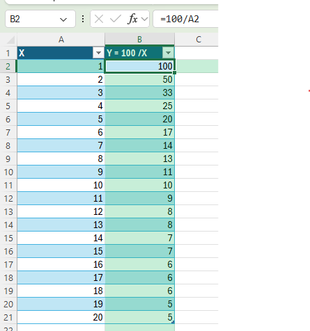
In A1, type X, and in B1, type Y = 100/X. In column A, enter values 1 through 20 (use =ROW(A1) and drag down if needed)

In B2, enter the formula =100/A2

Drag the formula down to B21

Now you have the raw dataset of X-values and their corresponding hyperbolic Y-values.

Step 2 – Insert the Chart

Select the range A1:B21

Go to the Insert tab

Choose Scatter Chart > Scatter with Smooth Lines

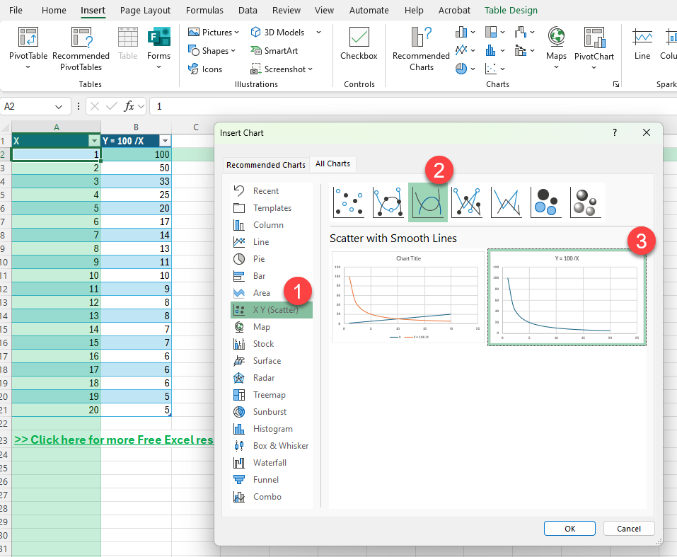
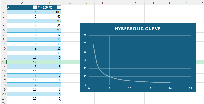
The chart now shows your inverse relationship.

Common Mistakes or Tips

Using Line Charts Instead of Scatter Plots

• Scatter plots are better for non-linear data with numeric X-values.

Forgetting Absolute References

• When referring to a constant, use $D$2, not D2, to lock the cell.

Dividing by Zero

• Never include 0 in your X-values. Use an IF formula like =IF(A2=0,"", $D$2/A2) if needed.

Overcrowding the Chart

• Stick with 10–30 points for clarity unless more precision is required.

Neglecting Labels

• Always label your axes and include a chart title for usability.

Bonus Tips and Advanced Scenarios

1. Add Data Labels Based on Conditions

If you only want to highlight specific points on the curve:

• Select your chart

• Click the data series, then Add Data Labels

• Right-click labels > Format > Custom Values

You can reference cells conditionally using helper columns.

2. Use Power Query to Import X Values

Automate your X-values from a CSV:

• Go to Data > Get & Transform Data > From Text/CSV

• Import your list of X-values

• In Power Query, add a column with formula =100 / [X]

• Load it back into your worksheet

This makes it easier to refresh data dynamically.

3. Use VBA to Auto-Fill Hyperbolic Values

Open the VBA Editor (Alt + F11), insert a module, and paste:

Sub InsertHyperbolicData()
Dim ws As Worksheet
Set ws = Sheets.Add
ws.Name = "Hyperbolic VBA"
ws.Range("A1").Value = "X"
ws.Range("B1").Value = "Y"
For i = 1 To 20
ws.Cells(i + 1, 1).Value = i
ws.Cells(i + 1, 2).Formula = "=100/A" & i + 1
Next i
End Sub

Run the macro to instantly populate a new sheet.

4. Highlight Thresholds with Conditional Formatting

Let’s say you want to highlight all Y-values below 10:

• Select column B

• Go to Home > Conditional Formatting > New Rule

• Choose Use a formula to determine which cells to format

• Use: =B2<10 and apply a color

5. Create a Dynamic Chart Title

Type this formula in F1:
="Hyperbolic Curve with A = "&D2

Then:

• Click the chart title

• In the formula bar, type =Sheet1!F1

Now your title updates when the constant changes.

FAQ

1. What is a hyperbolic curve used for in Excel?
It’s used to visualize inverse relationships, such as speed vs. time or cost per item vs. quantity.

2. Can I use a different formula like Y = A / (X + B)?
Yes, you can modify the formula to add constants or offsets. For example, =100/(A2+5) shifts the curve.

3. Why is my chart not smooth?
Use Scatter with Smooth Lines instead of Scatter with Straight Lines for a curved appearance.

4. Can I make this interactive?
Yes, by adding a constant cell and linking it in the formula, your curve can respond to user input.

5. What if I want to format large values better?
Use number formatting (Home > Number) or custom formats like #,##0.00 for readability.