Icon Sets In A Pivot Table

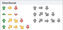
An Icon Set is a Conditional Formatting icon/graphic that you can include in your cells or Pivot Tables. The icon will depend on the cell´s value so you can highlight key variances or trends.

Key Takeaways

• Visually Enhance Your Pivot Table – Icon sets use symbols like arrows, traffic lights, or flags to represent value trends or performance at a glance.

• Conditional Formatting Integration – Icon sets are applied through conditional formatting, making it easy to layer visual cues on numerical data.

• Customize Thresholds and Rules – You can define what each icon represents by customizing value ranges, percentages, or formulas.

• Best for Comparison Metrics – Icon sets are ideal for quickly highlighting high, medium, and low values, helping users focus on what’s important.

• Works Dynamically with Pivot Updates – When your pivot table data changes or is refreshed, the icon sets update automatically to reflect the new values.

The Different Sets

There are a few sets that you can include, like:

DIRECTIONAL (Change in values)

SHAPES (Milestones)

INDICATORS (Positive/Negative)

RATINGS (Scores)

I show you how easy it is to insert an Icon Set within a Pivot Table that will show a “directional icon” depending on the change of the monthly sales values.

So when monthly sales increase from the previous month, a green up arrow is shown and when monthly sales decrease, a red down arrow is shown.

STEP 1: Place the SALES Field in VALUES

 

STEP 2: Click on the new field and Select Value Field Settings

Go to Show Values as > Difference From > (previous) to get the difference from the previous month

 

STEP 3: Click in a variance cell. Go to Home > Styles > Conditional Formatting > Icon Sets > The First Icon Set

STEP 4: Make sure to select the third option. This excludes the subtotals and grand totals.

 

STEP 5: Go to Home > Styles > Conditional Formatting > Manage Rules

Select Edit Rule.

Set the settings to the ones shown below. This will set the column to show the arrow icons only.

Your icons are now ready in your Pivot Table!

 

Frequently Asked Questions

How do I add icon sets to a Pivot Table?
Select the values in the Pivot Table, go to the “Home” tab, click “Conditional Formatting,” choose “Icon Sets,” and pick a style.

Can I apply icon sets to non-numeric fields?
No, icon sets only work on numeric values such as sales, percentages, or scores within your Pivot Table.

Do icon sets change when I refresh the Pivot Table?
Yes, icon sets are dynamic and will automatically update based on the new data values after a refresh.

Can I adjust which values trigger each icon?
Yes, you can edit the rule by going to Conditional Formatting > Manage Rules > Edit Rule, where you can set thresholds and icon logic.

Will the icons remain if I copy the Pivot Table elsewhere?
If you copy the Pivot Table with formatting, the icons will remain, but if you paste as values, the conditional formatting—including icons—will be lost.