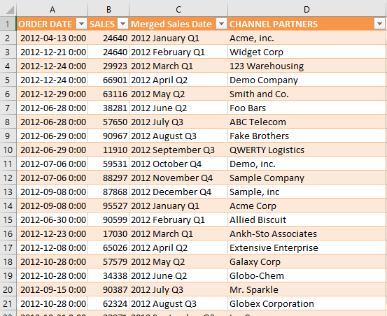
Power Query lets you perform a series of steps to transform your Excel data. One of the steps it allows you to take is to merge columns easily.
Normally I would use the CONCATENATE formula to merge columns together, however a cleaner way is to simply use Power Query for this.
Let’s go through the steps in detail:
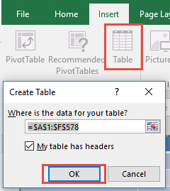
STEP 1: Select your data and turn it into an Excel Table by pressing the shortcut Ctrl + T or by going to Insert > Table
STEP 2: Go to Data > Get & Transform > From Table (Excel 2016) or Power Query > Excel Data > From Table (Excel 2013 & 2010)
Excel 2016:
Excel 2013 & 2010:
STEP 3: This will open up the Power Query Editor.
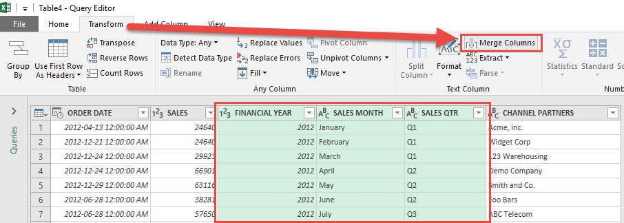
We want to merge the three columns: Financial Year, Sales Month, and Sales Qtr.
Select these three columns by clicking on the Financial Year heading, holding the Shift key and then clicking on the Sales Qtr heading.
Go to Transform > Merge Columns
STEP 4: This will open up the Merge Columns dialogue box.
In the Separator section, select Space.
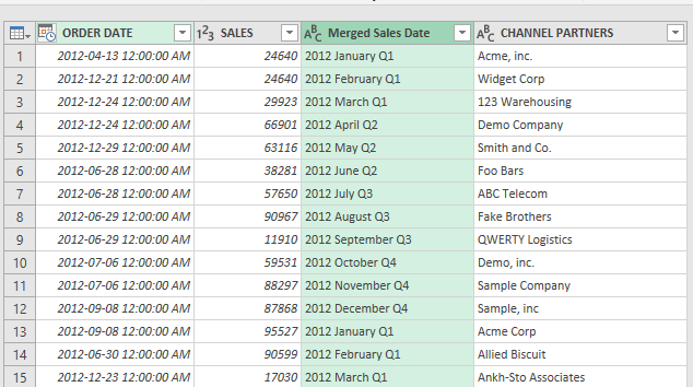
In the New column name, manually enter the name for this new column e.g. Merged Sales Data
Click OK.
Now you will see your changes take place.
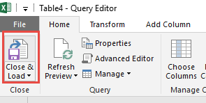
STEP 5: Click Close & Load from the Home tab and this will open up a brand new worksheet in your Excel workbook with the updated values.
You now have your new table in a new worksheet with the merged columns!

Bryan
Bryan Hong is an IT Software Developer for more than 10 years and has the following certifications: Microsoft Certified Professional Developer (MCPD): Web Developer, Microsoft Certified Technology Specialist (MCTS): Windows Applications, Microsoft Certified Systems Engineer (MCSE) and Microsoft Certified Systems Administrator (MCSA).
He is also an Amazon #1 bestselling author of 4 Microsoft Excel books and a teacher of Microsoft Excel & Office at the MyExecelOnline Academy Online Course.

