Predetermined Number Formatting in Excel Pivot Tables

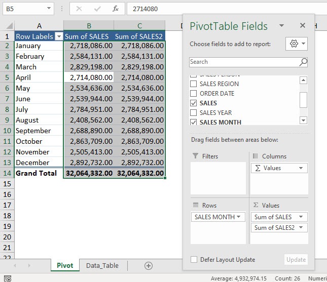
What happened? Why did your formatting not take effect on the second sales column? I have the perfect workaround for adding predetermined number formatting in Pivot Table. Read on below!

Exercise Workbook:

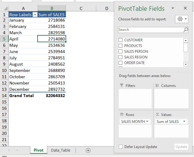
Here is our current Pivot Table setup:

STEP 1: Let us select the entire Pivot Table. Go to PivotTable Analyze > Actions > Select > Entire PivotTable

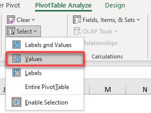
STEP 2: Now to select the sales numbers column, go to PivotTable Analyze > Actions > Select > Values

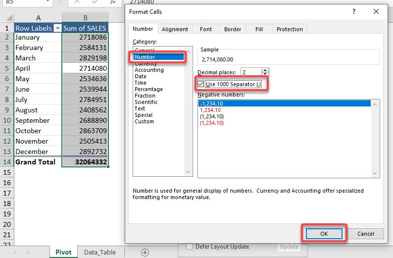
STEP 3: Let us apply our number formatting! Open the Format Cells dialog by pressing CTRL + 1

Select Number and tick the Use 1000 Separator (,)

Click OK

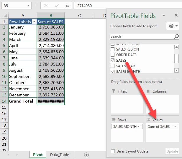
STEP 4: The number formatting is applied on our first Sales column. Now drag SALES to Values

The formatting is also applied to our second Sales column!

Bryan

Bryan Hong is an IT Software Developer for more than 10 years and has the following certifications: Microsoft Certified Professional Developer (MCPD): Web Developer, Microsoft Certified Technology Specialist (MCTS): Windows Applications, Microsoft Certified Systems Engineer (MCSE) and Microsoft Certified Systems Administrator (MCSA).

He is also an Amazon #1 bestselling author of 4 Microsoft Excel books and a teacher of Microsoft Excel & Office at the MyExecelOnline Academy Online Course.