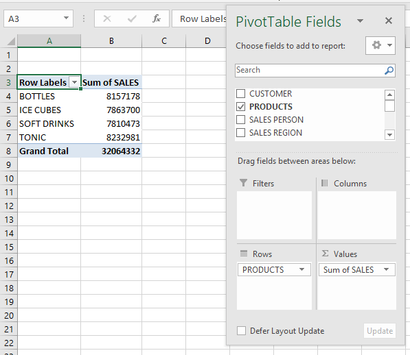
Did you know that Excel can automatically generate Pivot Tables for you? You heard that right, there are Recommended Pivot Tables in Excel that you can actually use! This is a new feature introduced in Excel 2013. Excel’s Recommended Pivot Tables feature is especially advantageous, simplifying the creation process and enabling users to focus on interpreting data rather than configuring it. By the end of this guide, you’ll be equipped to harness this tool’s full potential to make data-driven decisions confidently.
It is very simple to do so, and we will show you how!
Key Takeaways:
- Excel’s Recommended Pivot Tables suggest layout options based on your data automatically.
- This feature was introduced in Excel 2013 and is great for beginners and pros alike.
- Recommended Pivot Tables save time and reduce setup errors, making analysis quicker.
- You can easily modify suggested layouts, like switching from “Count” to “Sum.”
- They support advanced customization—from conditional formatting to external data integration.
Table of Contents
Unveiling Recommended Pivot Tables
What Are Recommended Pivot Tables?
Recommended Pivot Tables in Excel are an intuitive feature designed to simplify the creation of PivotTables by suggesting different layout options based on your dataset. This feature examines your data and automatically generates a selection of suitable PivotTable designs, allowing you to choose one that best meets your analytical needs. This functionality is particularly beneficial for those who may be new to PivotTables, as it eliminates much of the guesswork involved in setting up an effective data summary and visualization. Recommended Pivot Tables streamline the process, making it accessible for users of all skill levels.
Benefits of Using Recommended Pivot Tables
Opting for Recommended PivotTables offers several advantages that enhance Excel’s analytics capabilities. First and foremost, they save time by quickly suggesting appropriate layouts based on your specific data set—a feature particularly useful for beginners. These suggestions allow you to skip the complex setup process and dive right into data analysis. Moreover, Recommended PivotTables help ensure accuracy by providing layouts that align with your data structure. They also improve efficiency by removing much of the trial and error associated with traditional PivotTables. Additionally, they enhance data visualization by offering clear, concise ways to present your information. Ultimately, these benefits make Recommended PivotTables an invaluable tool for anyone looking to gain insights from their data efficiently.
Getting Started with Recommended Pivot Tables
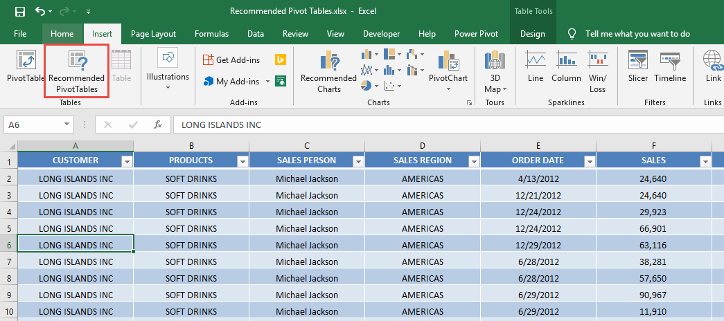
STEP 1: Make sure you have selected your data. Go to Insert > Tables > Recommended Pivot Tables
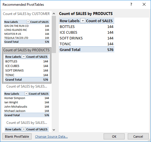
STEP 2: You will see the generated Pivot Table recommendations.
Let us select the Count of SALES by PRODUCTS. Click OK.
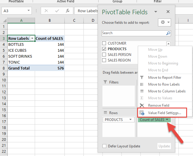
STEP 3: The generated Pivot Table is now in a new sheet. Let us make some changes to it.
Click on COUNT of SALES and select Value Field Settings.
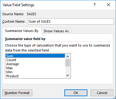
We want it to display the Total sum of Sales per Product instead. Select Sum and click OK.
With just that, your Pivot Table is now ready!
Tips for Maximizing PivotTable Efficiency
Customizing Layouts for Better Insights
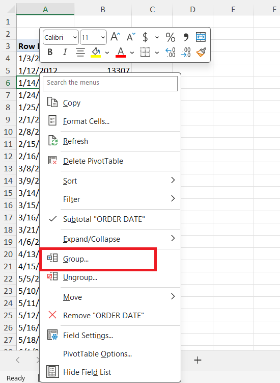
Customizing the layout of your Recommended PivotTables can significantly enhance your insights. Start by rearranging fields in the Rows, Columns, Values, and Filters areas in the PivotTable Field List to best reflect your analytical needs. Consider grouping dates or categorical variables for more cohesive data summaries.
Use the “Design” tab to explore layout options like Report Layouts and Subtotals to display data in a way that makes the most sense to you.
Additionally, you can add calculated fields or items to create custom calculations directly in the table.
Conditional formatting is another powerful tool to highlight critical data points or trends dynamically. By tailoring the layout, you enhance the readability and interpretability of the data, leading to more actionable insights.
Leveraging External Data Sources
Incorporating external data sources into your Recommended Pivot Tables can expand your analysis and provide a more comprehensive view of your data landscape. Begin by ensuring that your external data is in a compatible format, such as a CSV file, or accessible from a data connection. Use the “Data” tab in Excel to import these external datasets and integrate them into your workbook.
Next, establish relationships between your Excel tables if your dataset is stored across multiple tables. This allows for a more coherent analysis when using multiple tables. When building your PivotTable, ensure that the external data fields are correctly interpreted in conjunction with your existing data. By leveraging external sources, you enrich your datasets with additional context and information, enhancing the depth of your analysis and leading to more robust conclusions.
FAQs
What are Recommended PivotTables in Excel, and how do they work?
Recommended PivotTables are a feature in Excel that automatically analyzes your dataset and suggests various PivotTable layouts tailored to your data. It’s especially useful for users who are unfamiliar with building PivotTables from scratch. When you select your data and use this feature, Excel shows you several layout suggestions, like totals by category or counts by item. You simply pick the one that fits your needs and Excel creates it instantly.
Who should use Recommended PivotTables—are they only for beginners?
While beginners find them particularly helpful, Recommended PivotTables are not limited to newbies. Even advanced Excel users can benefit from them as a quick starting point for analysis. They help save time by skipping the manual configuration step and allowing users to jump directly into customizing and interpreting results. So, whether you’re a data novice or a seasoned analyst, this feature can speed up your workflow.
Can I customize a Recommended PivotTable after it’s created?
Absolutely. Once the PivotTable is generated, you can modify the fields, change summary types (like switching from Count to Sum), and adjust layouts. You can drag fields into different areas (Rows, Columns, Values, Filters) and even apply conditional formatting or calculated fields. This flexibility ensures you’re not stuck with Excel’s suggestion—you can mold it to fit your exact needs. It’s like a smart template you can tweak endlessly.
How do I create a Recommended PivotTable in Excel?
First, select your data range, then go to Insert > Tables > Recommended PivotTables. Excel will display several suggested layouts based on your data. Choose the one that best fits your analysis goal and click OK. The PivotTable will appear on a new sheet, and you can further customize it as needed using field settings and layout options.
Can I use external data with Recommended PivotTables?
Yes, you can enhance your PivotTables by incorporating external data sources like CSV files, databases, or online feeds. Start by importing the data into Excel through the Data tab. You may need to establish relationships between tables if you’re using multiple sources. Once the data is available in your workbook, it can be integrated into your PivotTables seamlessly, giving you a richer, multi-dimensional view of your dataset.

Bryan
Bryan Hong is an IT Software Developer for more than 10 years and has the following certifications: Microsoft Certified Professional Developer (MCPD): Web Developer, Microsoft Certified Technology Specialist (MCTS): Windows Applications, Microsoft Certified Systems Engineer (MCSE) and Microsoft Certified Systems Administrator (MCSA).
He is also an Amazon #1 bestselling author of 4 Microsoft Excel books and a teacher of Microsoft Excel & Office at the MyExecelOnline Academy Online Course.

