Reverse Rows Using Power Query

Power Query lets you perform a series of steps to transform your Excel data.  One of the steps it allows you to take is to reverse the order of rows very easily.

Download excel workbookReverse-Rows-2.xlsx

 

To provide a quick comparison, it’s not straightforward to reverse rows in Excel without Power Query:

We have our data that we want to reverse the row order:

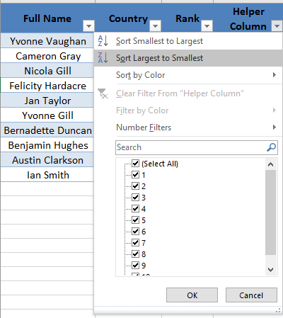
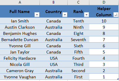
Since Excel does not have a Reverse Row function, we need to add a Helper column manually that has the order listed out (from 1 to 10).

We use the Sort function and select Sort Largest to Smallest.

The data is now in reverse order.

 

Let’s go through the steps in detail on how to do it easily in Power Query:

 

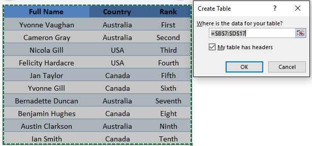
STEP 1: Select your data and turn it into an Excel Table by pressing the shortcut Ctrl + T or by going to Insert > Table

 

STEP 2: Go to Data > Get & Transform > From Table (Excel 2016) or Power Query > Excel Data > From Table (Excel 2013 & 2010)

Excel 2016:

 

Excel 2013 & 2010:

 

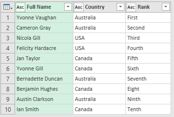
STEP 3: This will open up the Power Query Editor.

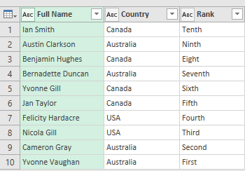
Currently you can see the Ranks ordered from First to Tenth. We want to reverse the ordering of the rows.

 

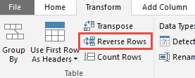
STEP 4: Within here you need to select Transform > Reverse Rows

 

STEP 5: Now you will see your changes take place. The Ranks are now ordered from Tenth to First.

 

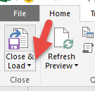
STEP 6: Click Close & Load from the Home tab and this will open up a brand new worksheet in your Excel workbook with the updated data.

You now have your new table in reverse order.