50 Things You Can Do With Excel Power Query

List of 50 Things You Can Do With Excel Power Query

Installing Power Query

1. How To Install Power Query in Excel 2010

Power Query is a new add-in that was introduced in Excel 2013 by Microsoft and was that popular that they made it backward compatible with Excel 2010.

So what is Power Query?

Well you know when you get data from a file, a data dump/import, or an external data source and it comes into Excel in an ugly, unworkable format? I can hear you say YEEEES!

Well Power Query accesses, cleans, and transforms all that messy data and displays it in a way that Excel loves and can work with. The best thing is that the next time you receive the same ugly file, all you need to do is press the Refresh button and your data will automatically be cleaned up and displayed the correct way!

So no more formulas, text to columns, trim spaces, vlookup, find & replace, etc.

You have all that functionality in Power Query at the press of a menu command! Now your life has just become a lot…well, a hell of a lot easier 🙂

Apart from cleaning data, Power Query can append or merge two separate tables together (bye bye VLOOKUP!) as well as create extra columns in your data that can display your custom calculations!

You can use Power Query to perform transformations that would be very complex in VBA or SQL. So goodbye VBA coding 🙂 🙂 🙂

So how do I get your hands on this super awesome add-in…I hear you say?

First, you need to have Microsoft Office 2010 Professional Plus with Software Assurance. If you do not have this then you will need to upgrade to Office 365 using this link:

https://products.office.com/en-us/home

 

STEP 1: The first step is to check the Excel bit version that you have on your PC.

To check the bit version, you need to go and open any Excel workbook and go to File > Help and on the far right-hand side, you will see the Version and the bit number in brackets, either (32-bit) or (64-bit). Once you know this, close out of Excel completely!

 

STEP 2: You will need to click on the following link and download the Power Query add-in from Microsoft’s website:

https://www.microsoft.com/en-us/download/details.aspx?id=39379

 

STEP 3: Press the Download button and you will need to select the download bit version based on the bit system your Excel 2010 version is running (from Step 1):

Press the NEXT button…

…and this will start the download of the add-in installer .msi file installer on your browser (if you do not see this, go to your browser’s Downloads folder).

 

STEP 4: Click on the .msi file to run the installer:

 

STEP 5: This will bring up the Microsoft Power Query for Excel Setup:

Click the Next button and accept the terms of the Licence Agreement and press Next again:

You will be asked in which destination folder you want to install the Power Query.

Click Next for the default folder or Change if you want to install it in another folder:

Click Next and select the Install button:

Click Yes if it asks you if you want to install Power Query on your computer. The install will now begin.

You will get the following message once your install has been completed successfully. Press Finish!

 

STEP 6: Open a blank Excel workbook and on the ribbon menu you should now see the Power Query tab:

 

STEP 7: If you do not see the Power Query tab you will need to activate this from the back end of Excel.

You will need to go to File > Options > Add-Ins > and at the bottom you will need to select the Manage drop-down and choose COM Add-ins and hit the Go button:

This will open the COM Add-Ins dialogue box and you will need to check the box for Microsoft Power Query for Excel and press OK.

You will now see Power Query on your ribbon!

 

 

2. Install Power Query With Excel 2013

Power Query is a new add-in that was introduced in Excel 2013 by Microsoft and was that popular that they made it backward compatible with Excel 2010.

So what is Power Query?

Well you know when you get data from a file, a data dump/import, or an external data source and it comes into Excel in an ugly, unworkable format? I can hear you say YEEEES!

Well Power Query accesses, cleans, and transforms all that messy data and displays it in a way that Excel loves and can work with. The best thing is that the next time you receive the same ugly file, all you need to do is press the Refresh button and your data will automatically be cleaned up and displayed the correct way!

So no more formulas, text to columns, trim spaces, vlookup, find & replace, etc.

You have all that functionality in Power Query at the press of a menu command! Now your life has just become a lot…well, a hell of a lot easier 🙂

Apart from cleaning data, Power Query can append or merge two separate tables together (bye bye VLOOKUP!) as well as create extra columns in your data that can display your custom calculations!

You can use Power Query to perform transformations that would be very complex in VBA or SQL. So goodbye VBA coding 🙂 🙂 🙂

So how do I get your hands on this super awesome add-in…I hear you say?

First you need to have Microsoft Office 2013. If you do not have this then you will need to upgrade to Office 365 using this link:

https://products.office.com/en-us/home

STEP 1: The first step is to check the Excel bit version that you have on your PC.

To check the bit version, you need to go and open any Excel workbook and go to File > Account > About Excel and from the pop up dialogue box you will see the bit number, either 32-bit or 64-bit. Once you know this, close out of Excel completely!

 

STEP 2: You will need to click on the following link and download the Power Query add-in from Microsoft’s website:

https://www.microsoft.com/en-us/download/details.aspx?id=39379

STEP 3: Press the Download button and you will need to select the download bit version based on the bit system your Excel 2013 version is running (from Step 1):

Press the NEXT button…

…and this will start the download of the add-in installer .msi file installer on your browser (if you do not see this, go to your browser’s Downloads folder).

STEP 4: Click on the .msi file to run the installer:

STEP 5: This will bring up the Microsoft Power Query for Excel Setup:

Click the Next button and accept the terms of the Licence Agreement and press Next again:

You will be asked in which destination folder you want to install Power Query.

Click Next for the default folder or Change if you want to install it in another folder:

Click Next and select the Install button:

Click Yes if it asks you if you want to install Power Query on your computer. The install will now begin.

You will get the following message once your install has been completed successfully. Press Finish!

STEP 6: Open a blank Excel workbook and on the ribbon menu you should now see the Power Query tab:

STEP 7: If you do not see the Power Query tab you will need to activate this from the back end of Excel.

You will need to go to File > Options > Add-Ins > and at the bottom you will need to select the Manage drop-down and choose COM Add-ins and hit the Go button:

This will open the COM Add-Ins dialogue box and you will need to check the box for Microsoft Power Query for Excel and press OK.

You will now see Power Query on your ribbon!

 

Data Cleanup & Transformation

3. Inventory Your Files

Power Query lets you perform a series of steps to transform your Excel data.

One of the possible steps that surprised me was that I could list out the files on my computer!

This is useful if you want to do some analysis on your file list (i.e. finding a file, checking which files have the biggest size to clear up space).

 

Let’s go through the steps in detail:

STEP 1: Go to Data > New Query > From File > From Folder

(In Excel 2010 & 2013 you need to go to Power Query > From File > From Folder)

 

STEP 2: Type in the path you want to list the files from. You can also browse for the folder. Click OK.

STEP 3: This will give you a preview of the file list. Click Edit to examine it more inside the Power Query editor.

STEP 4: You are now inside the Power Query Window.

You can add more information into your Table by clicking the Icon beside Attributes.

 

For example, we want to include the Size column. Uncheck (Select All Columns) and check Size. Click OK.

 

The size column is now shown.

 

STEP 5: Click Close & Load from the Home tab and this will automatically open up a brand new worksheet in your Excel workbook with the new data.

 

You now have your spanking new file list!

4. Keep Duplicate Records

Power Query or Get & Transform (In Excel 2016) lets you perform a series of steps to transform your Excel data. One of the steps allows you to take is to keep duplicate records.

We usually remove duplicated lines but if we need to keep and check what the duplicates are, Excel allows us to do that too!

Let’s suppose you have this set of data. You can see that the marked ones are duplicate values, let us keep them!

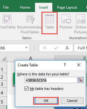
STEP 1: Select your data and turn it into an Excel Table by pressing the shortcut Ctrl + T or by going to Insert > Table

 

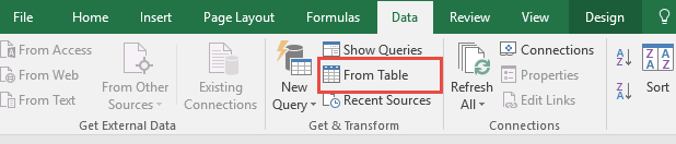
STEP 2: Go to Data > Get & Transform > From Table (Excel 2016) or Power Query > Excel Data > From Table (Excel 2013 & 2010)

Excel 2016:

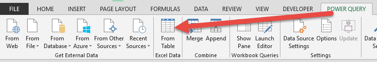
Excel 2013 & 2010:

 

STEP 3: This will open up the Power Query Editor.

Go to Home > Keep Rows > Keep Duplicates

 

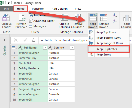
STEP 4: Click Close & Load from the Home tab and this will open up a brand new worksheet in your Excel workbook with the updated table.

You now have your new table with the duplicate rows kept!

How to Keep Duplicates in Excel

5. Split Column By Number of Characters

Power Query (in Excel 2010 & 2013) or Get & Transform (in Excel 2016) lets you perform a series of steps to transform your Excel data.

One of the steps it allows you to do is to split column by number of characters easily.

This is helpful when you have columns that you want to split by an equal number of characters, say ID numbers.

Let’s suppose you have the following source data below. We want to split it by 3 characters so we will have 4 parts for each ID.

Let us get to work!

STEP 1: Select your data and turn it into an Excel Table by pressing the shortcut Ctrl + T or by going to Insert > Table

 

STEP 2: Go to Data > Get & Transform > From Table (Excel 2016) or Power Query > Excel Data > From Table (Excel 2013 & 2010)

Excel 2016:

Excel 2013 & 2010:

 

STEP 3: This will open up the Power Query Editor.

Select the column you want to split.

Go to Home > Split Column > By Number of Characters

 

STEP 4: Select 3 for the Number of characters, Split Repeatedly, and click OK.

STEP 5: Click Close & Load from the Home tab and this will open up a brand new worksheet in your Excel workbook with the updated table.

You now have your new table with the separated columns!

How to Split Column by Number of Characters in Excel

6. Duplicate Columns

Power Query (in Excel 2010 & 2013) or Get & Transform (in Excel 2016) lets you perform a series of steps to transform your Excel data.

One of the steps it allows you to do is to duplicate columns easily.

This is helpful when you have columns that you want to duplicate & make some temporary/permanent changes to it in the Query Editor but not in your source data.

Let’s suppose you have the following source data below. You can see that the marked column is the one we want duplicated, so let us get to work!

STEP 1: Select your data and turn it into an Excel Table by pressing the shortcut Ctrl + T or by going to Insert > Table

 

STEP 2: Go to Data > Get & Transform > From Table (Excel 2016) or Power Query > Excel Data > From Table (Excel 2013 & 2010)

Excel 2016:

Excel 2013 & 2010:

 

STEP 3: This will open up the Power Query Editor.

Select the column you want to duplicate.

Go to Add Column > General > Duplicate Column

 

STEP 4: Click Close & Load from the Home tab and this will open up a brand new worksheet in your Excel workbook with the updated table.

You now have your new table with the column duplicated!

 

Duplicate Columns Using Power Query or Get & Transform:

 

7. Use First Row as Headers

Power Query or Get & Transform (In Excel 2016) lets you perform a series of steps to transform your Excel data.

One of the steps it allows you to do is to use the first row as headers.

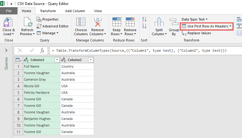
Let’s suppose you have this set of data below. You can see that the headers are not meaningful to us (Column1, Column2, Column3) so we want to eliminate them and replace them with the first row’s text (Full Name, Country, Rank):

STEP 1: Select your data and turn it into an Excel Table by pressing the shortcut Ctrl + T or by going to Insert > Table

 

STEP 2: Go to Data > Get & Transform > From Table (Excel 2016) or Power Query > Excel Data > From Table (Excel 2013 & 2010)

Excel 2016:

Excel 2013 & 2010:

 

STEP 3: This will open up the Power Query Editor.

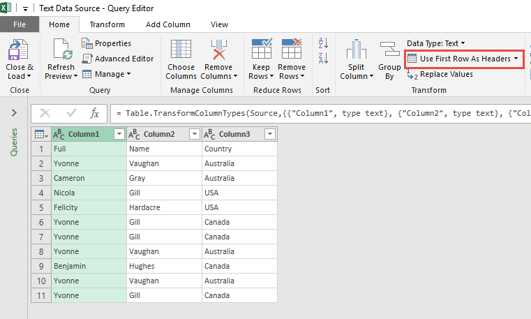
We want to change the Table headers with the first row. Go to Home > Use First Row As Headers

 

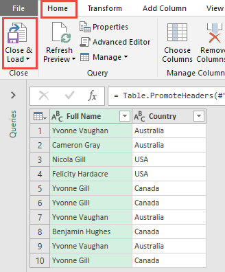
STEP 4: Click Close & Load from the Home tab and this will open up a brand new worksheet in your Excel workbook with the cleaned table.

You now have your new table with the brand new table header!

How to Use First Row as Headers Using Power Query or Get & Transform

8. Remove Columns

Power Query (in Excel 2010 & 2013) or Get & Transform (in Excel 2016) lets you perform a series of steps to transform your Excel data.

One of the steps it allows you to do is to remove columns easily.

This is helpful when you have columns that you want to eliminate and do not need in your final report – but do want to keep in your source data.

Let’s suppose you have the following source data below. You can see that the marked column is the one we want removed, so let us get rid of it!

STEP 1: Select your data and turn it into an Excel Table by pressing the shortcut Ctrl + T or by going to Insert > Table

 

STEP 2: Go to Data > Get & Transform > From Table (Excel 2016) or Power Query > Excel Data > From Table (Excel 2013 & 2010)

Excel 2016:

Excel 2013 & 2010:

 

STEP 3: This will open up the Power Query Editor.

Select the column(s) you want to remove. TIP: Hold the CTRL key to select multiple columns.

Go to Home > Remove Columns > Remove Columns

 

STEP 4: Click Close & Load from the Home tab and this will open up a brand new worksheet in your Excel workbook with the cleaned table.

You now have your new table with the column removed!

9. Remove Duplicates

Power Query or Get & Transform (In Excel 2016) lets you perform a series of steps to transform your Excel data. One of the steps it allows you to take is to remove duplicates easily. This removes the human error whenever you try to delete your duplicate data manually!

Let’s suppose you have this set of data. You can see that the marked ones are duplicate values, let us get rid of them!

STEP 1: Select your data and turn it into an Excel Table by pressing the shortcut Ctrl + T or by going to Insert > Table

 

STEP 2: Go to Data > Get & Transform > From Table (Excel 2016) or Power Query > Excel Data > From Table (Excel 2013 & 2010)

Excel 2016:

Excel 2013 & 2010:

 

STEP 3: This will open up the Power Query Editor.

Go to Home > Remove Rows > Remove Duplicates

 

STEP 4: Click Close & Load from the Home tab and this will open up a brand new worksheet in your Excel workbook with the cleaned table.

You now have your new table with the duplicate rows removed!

10. Fill Down Values

Power Query lets you perform a series of steps to transform your Excel data. One of the steps it allows you to take is to fill data down easily.

You might be wondering when you might need to fill the data down in your table.

Let’s suppose you have this set of data:

A lot of values are missing in the Sales Quarter column! It would be a lot of effort to input them one by one.

Let us sort the Sales Month, then the Sales Quarter column to get a better understanding:

You can see that we have at least one sales quarter populated for each month.

The technique here is that the Fill Down will copy the value directly above the empty cell and then fill it down the succeeding empty cell.

You can see from the arrows what will happen once we use Fill Down in Power Query.

Now that you know what our game plan is, let us get started!

 

STEP 1: Select your data and turn it into an Excel Table by pressing the shortcut Ctrl + T or by going to Insert > Table

 

STEP 2: Go to Data > Get & Transform > From Table (Excel 2016) or Power Query > Excel Data > From Table (Excel 2013 & 2010)

Excel 2016:

Excel 2013 & 2010:

 

STEP 3: This will open up the Power Query Editor.

A) Sort the Sales Month by Ascending order.

B) Then sort the Sales Quarter by Descending order.

Our data is now ready for the Fill down step.

 

STEP 4: Make sure the Sales Quarter column is selected. Go to Transform > Fill > Down

 

The missing values are now populated!

 

STEP 5: Click Close & Load from the Home tab and this will open up a brand new worksheet in your Excel workbook with the updated values.

 

You now have your new table with the updated values.

11. Create Index Columns

Power Query lets you perform a series of steps to transform your Excel data. One of the most common steps I do, is I want to add an index column that serves as a row counter of my data.

There is an alternative method of using the ROW formula in Excel.

However, if we simply want to keep it as a temporary column for data analysis, we can generate the Row Numbers using Power Query.

Thankfully Power Query has an option that allows us to create Index Columns!

 

Let’s go through the steps in detail:

STEP 1: Our sample data consists of Months and multiple Sales values for each quarter. Let us say we want a column that counts from 1 to 12 next to our data to serve as our row numbers.

(Make sure that your data is first converted into an Excel Table by pressing CTRL+T and OK).

Go to Data > Get & Transform > From Table (Excel 2016) or Power Query > Excel Data > From Table (Excel 2013 & 2010)

Excel 2016:

Excel 2013 & 2010:

 

STEP 2: This will open up the Power Query Editor.

Within here you need to select Add Column > Add Index Column > Custom

 

STEP 3: This brings up the Index Column dialogue box.

Set the Starting Index into 1, this would mean the starting number will be 1.

For the Increment, place in 1. This means that every succeeding number will be incremented by one. So we will have 1, 2, 3, 4 and so on..

Click OK.

 

STEP 4: Now you will see your changes take place and the data now has an index column!

 

STEP 5: Click Close & Load from the Home tab and this will automatically open up a brand new worksheet in your Excel workbook with the new data.

You now have your new table with your index column!

12. Remove Rows With Errors

Power Query lets you perform a series of steps to transform your messy Excel data.

One of the most common steps I do, is to clean my data and remove rows that have erroneous data, like this:

Thankfully Power Query has an option that allows us to remove rows with errors!

 

Let’s go through the steps in detail:

STEP 1: Our sample data contains the Sales numbers for each month. However, you can see that there are some months (4 of them) that have invalid data. We want to remove these rows.

Go to Data > Get & Transform > From Table (Excel 2016) or Power Query > Excel Data > From Table (Excel 2013 & 2010)

Excel 2016:

Excel 2013 & 2010:

 

STEP 2: This will open up the Power Query Editor.

 

Within here you need to click the Table icon on the upper left-hand corner of the table.

Then select Remove Errors.

 

STEP 3: Now all of the rows with errors will be removed from the table.

 

STEP 4: Click Close & Load from the Home tab and this will open up a brand new worksheet in your Excel workbook with the new data.

 

You now have your new Excel table without any erroneous rows!

13. Create Pivot Columns

Power Query lets you perform a series of steps to transform your Excel data. One of the most common steps I do, is I want to simplify my data and aggregate them together into something like this:

Thankfully Power Query has an option that allows us to create Pivot Columns!

 

Let’s go through the steps in detail:

STEP 1: Our sample data consists of Sales Quarter and multiple sales values for each quarter. We want to sum them all upper quarter. Let us load our data into Power Query.

(Make sure that your data is first converted into an Excel Table by pressing CTRL+T and OK).

Go to Data > Get & Transform > From Table (Excel 2016) or Power Query > Excel Data > From Table (Excel 2013 & 2010)

Excel 2016:

Excel 2013 & 2010:

 

STEP 2: This will open up the Power Query Editor.

Within here you need to select Transform > Pivot Column

 

 

STEP 3: This brings up the Pivot Column dialogue box.

For the Values Column drop-down, select the column name from our data that has the values in it…in our example it will be SALES.

Click on advanced options and this will bring up the Aggregate Value Function. Here we select how the new cells should be combined.

As we want to show the Sales Totals for each quarter, we need to select the Sum option from the drop-down box.

Click OK.

 

STEP 4: Now you will see your changes take place and the data has now been grouped and summed!

 

STEP 5: Click Close & Load from the Home tab and this will automatically open up a brand new worksheet in your Excel workbook with the new data.

 

You now have your new table with the total of each sales quarter. That’s why they call it POWER QUERY!!!

14. Group Rows and Get Counts

Power Query lets you perform a series of steps to transform your Excel data.

One of the steps it allows you to take is to group rows and get the counts of each group very easily.

Download excel workbookGroup-By-Count.xlsx

Let’s go through the steps in detail:

 

STEP 1: Select your data and turn it into an Excel Table by pressing the shortcut Ctrl + T or by going to Insert > Table

 

STEP 2: Go to Data > Get & Transform > From Table (Excel 2016) or Power Query > Excel Data > From Table (Excel 2013 & 2010)

Excel 2016:

Excel 2013 & 2010:

 

STEP 3: This will open up the Power Query Editor.

We want to group this data by Country and show how many times each Country appeared in the table. (i.e. Australia appears 4 times in this table)

 

STEP 4: Within here you need to select Transform > Group By

 

STEP 5: Make sure to select Country for Group By, and select Count Rows for the Operation.

This will group your table by Country value, and count the number of occurrences of each country.

For example, the country of Australia appears 4 times in our table.

STEP 6: Now you will see your changes take place. And the data has now been grouped together.

 

STEP 7: Click Close & Load from the Home tab and this will open up a brand new worksheet in your Excel workbook with the new data.

You now have your new table with the counts of each country.

15. Reverse Rows

Power Query lets you perform a series of steps to transform your Excel data. One of the steps it allows you to take is to reverse the order of rows very easily.

Download excel workbookReverse-Rows-2.xlsx

 

To provide a quick comparison, it’s not straightforward to reverse rows in Excel without Power Query:

We have our data that we want to reverse the row order:

Since Excel does not have a Reverse Row function, we need to add a Helper column manually that has the order listed out (from 1 to 10).

We use the Sort function and select Sort Largest to Smallest.

The data is now in reverse order.

 

Let’s go through the steps in detail on how to do it easily in Power Query:

 

STEP 1: Select your data and turn it into an Excel Table by pressing the shortcut Ctrl + T or by going to Insert > Table

 

STEP 2: Go to Data > Get & Transform > From Table (Excel 2016) or Power Query > Excel Data > From Table (Excel 2013 & 2010)

Excel 2016:

Excel 2013 & 2010:

 

STEP 3: This will open up the Power Query Editor.

Currently, you can see the Ranks ordered from First to Tenth. We want to reverse the ordering of the rows.

 

STEP 4: Within here you need to select Transform > Reverse Rows

 

STEP 5: Now you will see your changes take place. The Ranks are now ordered from Tenth to First.

 

STEP 6: Click Close & Load from the Home tab and this will open up a brand new worksheet in your Excel workbook with the updated data.

You now have your new table in reverse order.

16. Transpose

Power Query lets you perform a series of steps to transform your Excel data. One of the steps it allows you to take is to transpose data very easily.

Transposing a data table is basically rotating your data from rows to columns, or from columns to rows. To further explain this concept, screenshots are provided below.

Download excel workbookTranspose.xlsx

 

Let’s go through the steps in detail:

STEP 1: Select your data and turn it into an Excel Table by pressing the shortcut Ctrl + T or by going to Insert > Table

 

STEP 2: Go to Data > Get & Transform > From Table (Excel 2016) or Power Query > Excel Data > From Table (Excel 2013 & 2010)

Excel 2016:

Excel 2013 & 2010:

 

STEP 3: This will open up the Power Query Editor.

We want to rotate this data from rows to columns.

 

STEP 4: Within here you need to select Transform > Transpose

 

STEP 5: Now you will see your changes take place.

 

STEP 6: Click Close & Load from the Home tab and this will open up a brand new worksheet in your Excel workbook with the transposed data.

You now have your new transposed table.

17. Replace Values

 

Power Query lets you perform a series of steps to transform your Excel data. One of the steps it allows you to take is to replace values easily.

Download excel workbookReplace-Values.xlsx

 

Let’s go through the steps in detail:

STEP 1: Select your data and turn it into an Excel Table by pressing the shortcut Ctrl + T or by going to Insert > Table

 

STEP 2: Go to Data > Get & Transform > From Table (Excel 2016) or Power Query > Excel Data > From Table (Excel 2013 & 2010)

Excel 2016:

Excel 2013 & 2010:

 

STEP 3: This will open up the Power Query Editor.

We want to change the Country Australia into New Zealand. Make sure you have the Country column selected by clicking on the Country header.

 

STEP 4: Within here you need to select Transform > Replace Values

 

STEP 5: This will open up the Replace Values dialogue box.

Place Australia in Value to Find, and New Zealand in Replace With. This will replace all of the Australia values with New Zealand.

Click OK.

STEP 6: Now you will see your changes take place.

 

STEP 7: Click Close & Load from the Home tab and this will open up a brand new worksheet in your Excel workbook with the updated values.

You now have your new table with the updated values.

18. Split First & Last Name

There are times when you receive a data set of employee full names in one column and you want to separate the full name into first name and surname in separate columns.

This is a common task and most people may refer to complex formulas to do this and waste lots of time in the process.

With Power Query, you can split the full name that is in one cell into separate columns with just a few mouse clicks.

Here is how…

Download excel workbookSplit-Columns-First-Last-Name.xlsx

STEP 1: Click in your data and turn it into an Excel Table by pressing the shortcut CTRL+T or by going to Insert Table

 

STEP 2: Go to Power Query > From Table

 

STEP 3: This will open up the Power Query Editor. Within here you need to select Home > Split Columns > By Delimiter

 

STEP 4: This will open up the Split Column by Delimiter dialogue box.

In the drop down box under Select or enter delimiter you need to choose Space

STEP 5: For the Split option, you need to select the default At each occurrence of the delimiter (since there is only one space in each cell’s data) and press OK

This will split the full name into two separate columns, one for the first name called FULL NAME.1 and another for the surname called FULL NAME.2

 

STEP 6: Now all you need to do is press Close & Load from the Home tab and this will open up a brand new worksheet in your Excel workbook with the split columns

You can amend the column headings and here you have your full name split into separate columns…Easy hey!

19. Consolidate Multiple Excel Workbooks

One of the most sought after query from the millions of Excel users around the world is:

How do I consolidate multiple Excel workbooks into one?

There are a couple of ways you can do this, using VBA or complex formulas but the learning curve is steep and out of reach for most Excel users.

Luckily with Power Query, this consolidation task can be done in a couple of minutes! That’s right, only a couple of minutes.

I show you how below…

Download excel workbookConsolidate-Multiple-Excel-Workbooks.xlsx

STEP 1: Create a New Folder on your Desktop or any directory and name it to whatever you like e.g. 2016 Sales

Move an Excel Workbook in this Folder that contains your Sales data e.g. January 2016.xlsx

 

STEP 2: Open a NEW Excel Workbook and go to Power Query > From File > From Folder

 

STEP 3: From the Folder dialogue box, click the Browse button

This will bring up the Browse for Folder dialogue box and you need to select the folder you created in Step 1 and press OK

 

STEP 4: This will open up the Query Editor.

From in here you need to select the first 2 columns (hold down the CTRL key to select) and Right Click on the column heading and choose Remove Other Columns

 

STEP 5: You need to go to Add Column > Add Custom Column

 

STEP 6: This will bring up the Add Custom Column dialogue box.

In here you need to name the new column E.G. Import, and within the Custom Column Formula you need to enter the following formula:

= Excel.Workbook([Content])

This will import the workbooks from within the Folder that you selected in Step 3

 

STEP 7: You now have a new column called Import.

Click on the Expand Filter and select the Data box only and press OK. This will import the workbook from the folder

 

STEP 8: Click on the Expand Filter from the Import.Data column and select OK. This imports all the columns’ data from within the workbook

 

STEP 9: Now it is time to transform the data by making some cosmetic changes!

Remove the Content column by Right Clicking and choosing Remove

 

STEP 10: Select the Import.Data.Column1 and filter out the CUSTOMER heading and press OK. This will also remove the other column’s headers

 

STEP 11: Select the Date column and go to Transform > Data Type > Date

 

STEP 12: Select the Sales column and go to Transform > Data Type > Currency

 

STEP 13: Rename the column headings to whatever you like by double clicking on the column header, renaming and pressing OK

 

STEP 14: Go to File > Close & Load.

 

This will put the data into a new worksheet within your workbook

 

STEP 15: You can now Insert a Pivot Table to do your analysis by going to Insert > Pivot Table > New/Existing Worksheet

 

Put the Months in the ROWS and the Sales $ in the VALUES area:

 

STEP 16: NOW FOR THE COOL PART!!!!

You can move similar workbooks into the Folder we created in Step 1, say for subsequent months eg. February 2016.xlsx, March 2016.xlsx etc

NB: The Excel Workbooks have to have the same format and number of columns as in the workbook we imported in Step 1

 

STEP 17: In your Excel workbook, click on the imported data and this will open up the Workbook Queries pane (If this does not open, go to Power Query > Show Pane)

Click the Refresh button (or you can go to Table Tools > Query > Refresh)

 

STEP 18: This will import the February 2016.xlsx and March 2016.xlsx data into the Excel workbook and append it to January’s data

STEP 19: Now you can Refresh the Pivot Table and the new imported data will be reflected

 

Next month all you have to do is drop in the new month’s workbook into the 2016 Sales Folder and Refresh the Query & the Pivot Table to see the results!

THAT IS POWER!!!!

20. Consolidate Multiple Excel Sheets

Power Query is awesome!

You will see why after viewing this Power Query tutorial.

I get lots of queries from my blog readers asking me if there is a way to easily consolidate multiple Excel worksheets into one.

With Power Query, the answer is YES!

If you have multiple Excel worksheets that are in the same format and their underlying differences are their values and dates (e.g. January Sales List, February Sales List, March Sales List, etc), then we can easily consolidate all the worksheets into one.

Here is how…

Download excel workbookAppend-Multiple-Sheetsv2.xlsx

STEP 1: Make sure that each worksheet´s data is in an Excel Table by clicking in the data and pressing CTRL+T

 

STEP 2: Click in each of the worksheets data that you want to consolidate and select:

Power Query > From Table

 

STEP 3: This will open up the Query Editor and all you have to do here is press Close & Load.

NB: Make sure to do Step 2 & 3 for each worksheet you want to consolidate

 

STEP 4: Select Power Query > Append

 

STEP 5: Choose the Three or more tables option

 

STEP 6: Add the tables to append from the Available Tables (from the left) to the Tables to Append (to the right) by selecting and pressing the Add button.

You can also organise the order that you want your consolidated table to appear by moving the Tables up or down

Press the OK button!

 

STEP 7: This will open up the Query Editor once again. Choose Close & Load.

 

STEP 8: This will open up a brand new worksheet which will consolidate all the worksheets into one big Table:

 

STEP 9: From this consolidate worksheet you can Insert a Pivot Table and do your analysis:

 

21. Unpivot Data Using Excel Power Query

In Excel 2016 it comes built in the Ribbon menu under the Data tab and within the Get & Transform group.

Power Query allows you to extract data from any source, clean and transform the data and then load it to another sheet within Excel, Power Pivot, or the Power BI Designer canvas.

One of the best features is to Unpivot Columns.

What that does is transforms columns with similar characteristics (e.g. Jan, Feb, March…) and puts them in a unique column or tabular format (e.g. Month), which then allows you to do further analysis using Pivot Tables which was not possible before unpivoting.

Here is how this is done:

Download excel workbookUnpivot.xlsx

STEP 1: Highlight your data and go to Power Query > From Table > OK

 

STEP 2: This opens the Power Query editor and from here you need to select the columns that you want to unpivot

STEP 3: You then need to go to the Transform tab and select Unpivot Columns

STEP 4: Go to the File tab and choose Close & Load

STEP 5: This will load and open the unpivoted data into a new worksheet with your Excel workbook. Now you can go crazy with your super analytical work, using Pivot Tables etc

22. Filter Records

Power Query or Get & Transform (In Excel 2016) lets you perform a series of steps to transform your Excel data. One of the steps it allows you to take is to filter records.

And the best part is, we will use an OR condition! It’s not that straightforward to do in Excel, but it’s magical in Power Query!

Let’s suppose you have this set of data below.

We want to filter records that starts with the letter “Y” OR has a country of “USA”. You can see that the marked ones are our targets, let us keep them!

STEP 1: Select your data and turn it into an Excel Table by pressing the shortcut Ctrl + T or by going to Insert > Table

 

STEP 2: Go to Data > Get & Transform > From Table (Excel 2016) or Power Query > Excel Data > From Table (Excel 2013 & 2010)

Excel 2016:

Excel 2013 & 2010:

 

STEP 3: This will open up the Power Query Editor.

Go to Filter Arrow of Full Name and select Text Filters > Begins With

Here is where the magic happens! Select Advanced and make sure your conditions are:

Full Name begins with Y

Or Country equals USA

Click OK.

 

STEP 4: Click Close & Load from the Home tab and this will open up a brand new worksheet in your Excel workbook with the updated table.

You now have your new table with the filtered rows kept!

How to Filter Records in Excel

Importing Data

23. Import Web Data

 

Power Query lets you clean and transform your raw & messed up data into a format where you can do further Excel analysis with ease.

Firstly, we would need data to play with Power Query, right? The good thing with Power Query is that there is a multitude of ways to pull in data.

One ways is to get data from the internet by using the importing web data feature. I will show you how we can parse a webpage and use it for Power Query!

 

Let’s go through the steps in detail using Excel 2016 as our workbook:

STEP 1: Go to Data > New Query > From Other Sources > From Web.

(In Excel 2010 & 2013 you need to go to Power Query > From Web)

 

STEP 2: This will ask for a website where you want to get the data from.

We want to get the stock market indexes from Google finance.

Copy and paste this URL: https://www.google.com/finance

Press OK to continue

 

STEP 3: Power Query will now try to parse this webpage, and in doing so, has determined that there are multiple tables of data in there.

Here is what Power Query brings back as Table options:

By clicking on the Table options in the Navigator pane, you will get a preview of the web data on the right-hand side.

Let’s select Table 0 for our example and press Edit.

 

STEP 4: The data is now imported into the Query Editor window.

 

STEP 5: We are going to transform Column3 so the data can be easier to analyze.

Select the Column3 heading with your mouse and go to Home > Split Column > By Delimiter.

 

STEP 6: We want to split the third column into two separate values. One for the actual number, and another for the percentage.

To achieve this, we need to split the data by the space in between the two values.

Select Space from the delimiter drop-down and press OK.

 

STEP 7: Our imported web data has been transformed into our liking.

 

We are now ready to load it into our Excel worksheet by selecting Close & Load

 

STEP 8: Now that the data is in your Excel worksheet, tomorrow all you need to do is select the data & press the Refresh button from the Workbook Queries pane on the right hand side.

 

You will have the latest stock prices & all this without copying and pasting from the webpage! Thank You Power Query 🙂

24. Import Data from XML

Power Query or Get & Transform (In Excel 2016) lets you perform a series of steps to transform your Excel data.

But what if your data source is not in your Excel spreadsheet?

It’s very common nowadays to get data imported from a company’s accounting or sales system in the XML format. If it’s inside a XML (extensible markup language) file, it’s very easy to import data from xml and right into Power Query!

Let’s suppose you have this set of data from the xml file:

STEP 1:

Using Excel 2016 (screenshot below)

Go to Data > New Query > From File > From XML

Using Excel 2013 or Excel 2010

Go to Power Query > From File > From XML

Select the xml file that contains the data. Click Import.

Select the XML Data Source. A preview of the xml data will be shown. If it looks good, press Edit.

 

STEP 2: This will open up the Power Query Editor. You can now perform your data manipulation here but we will keep the data as is.

Click Close & Load from the Home tab and this will open up a brand new worksheet in your Excel workbook with the imported table.

You now have your new table from the XML file!

Import Data from XML in Excel

25. Import Data from CSV

Power Query or Get & Transform (In Excel 2016) lets you perform a series of steps to transform your Excel data.

But what if your data source is not in your Excel spreadsheet but located on your desktop?

If it’s inside a CSV file – Comma Separated Values which is denoted by a .csv file extension & where the columns are separated by commas – it’s very easy to import data from csv and right into Power Query!

It’s very common nowadays to get data in the comma-delimited format.

Let’s suppose you have this set of data from the csv file:

STEP 1:

Using Excel 2016 (screenshot below)

Go to Data > New Query > From File > From CSV

Using Excel 2013 or Excel 2010

Go to Power Query > From File > From CSV

 

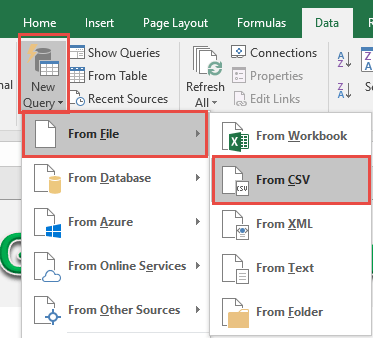
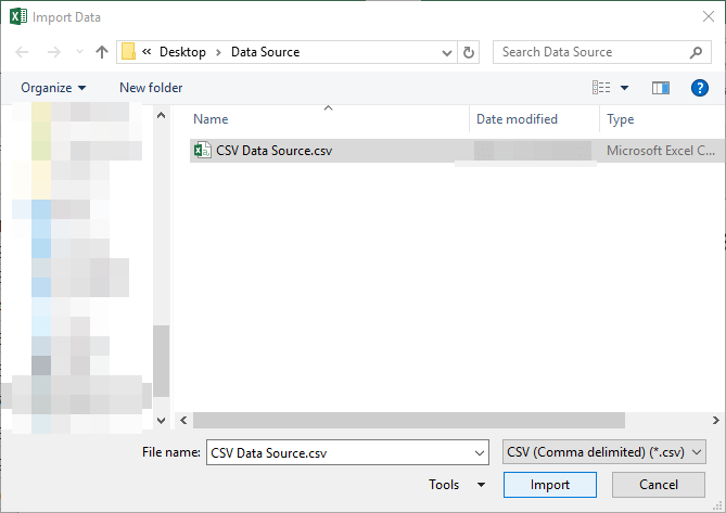
Select the csv file that contains the data. Click Import.

 

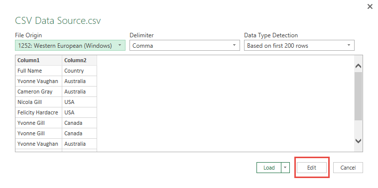
A preview of the csv data will be shown. If it looks good, press Edit.

 

STEP 2: This will open up the Power Query Editor.

Go to Home > Transform > Use First Row As Headers.

This will give your table the correct Column Headers.

 

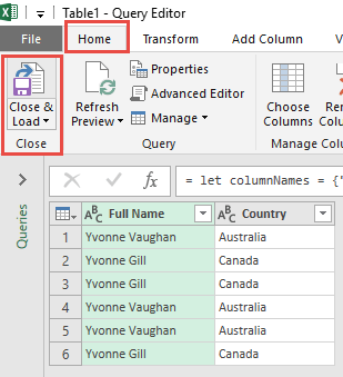
STEP 3: Click Close & Load from the Home tab and this will open up a brand new worksheet in your Excel workbook with the imported table.

You now have your new table from the csv file!

Import Data from CSV in Excel

26. Import Data from Text

Power Query or Get & Transform (In Excel 2016) lets you perform a series of steps to transform your Excel data.

But what if your data source is not in your Excel spreadsheet?

If it’s inside a text file, it’s very easy to import data from text and right into Power Query!

Let’s suppose you have this set of data from a text file:

STEP 1:

Using Excel 2016 (screenshot below)

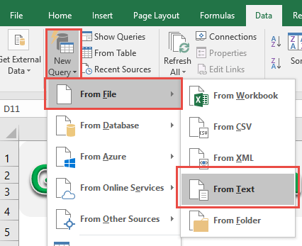
Go to Data > New Query > From File > From Text

Using Excel 2013 or Excel 2010

Go to Power Query > From File > From Text

 

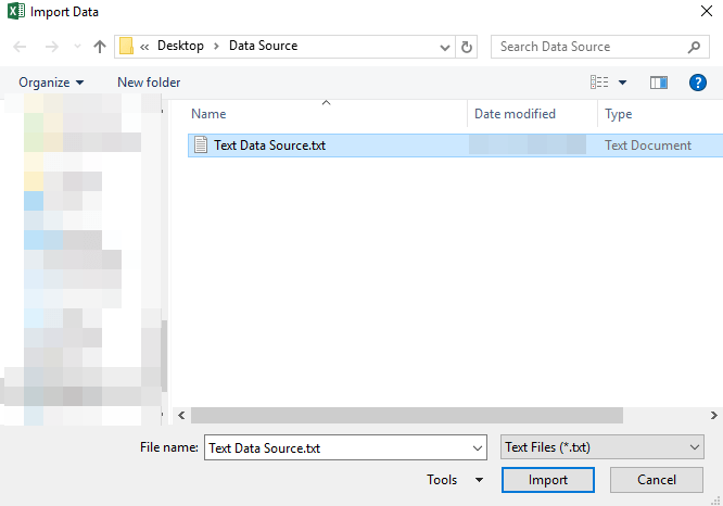
Select the text file (with extension .txt) that contains the data. Click Import.

 

A preview of the text data will be shown. If it looks good, press Edit.

 

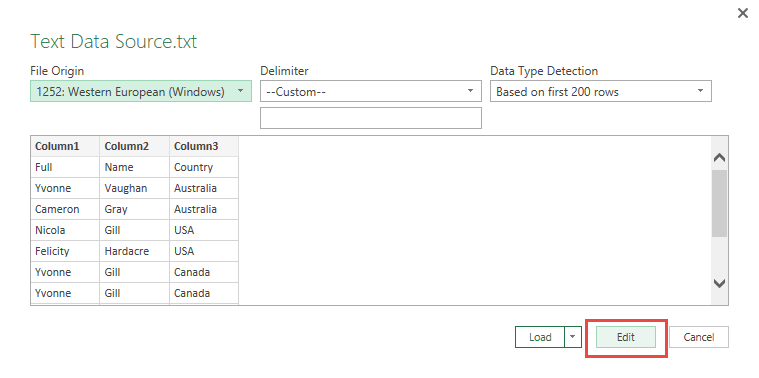
STEP 2: This will open up the Power Query Editor.

Go to Home > Transform > Use First Row As Headers.

This will give your table the correct Column Headers.

 

STEP 3: Click Close & Load from the Home tab and this will open up a brand new worksheet in your Excel workbook with the imported table.

 

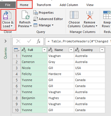
You now have your new table from the text file!

 

Import Data from Text Using Power Query or Get & Transform

The M Language

27. Getting Started with M

 

Power Query lets you perform a series of steps to transform your Excel data.

There are times when we want to do things that are not built in the user interface. This is possible with Power Query’s programming language, which is M.

To start off, we will do a simple example of merging the first name and second name into a new column. This is possible with the CONCATENATE formula, however I want to use a simple example for you to get a feel of how to use M in Power Query. Baby steps!

 

Let’s go through the steps in detail:

STEP 1: Select your data and turn it into an Excel Table by pressing the shortcut Ctrl + T or by going to Insert > Table

 

STEP 2: Go to Data > Get & Transform > From Table (Excel 2016) or Power Query > Excel Data > From Table (Excel 2013 & 2010)

Excel 2016:

Excel 2013 & 2010:

 

STEP 3: This will open up the Power Query Editor.

Here we will have our first taste of using M!

Go to Add Column > Add Custom Column

 

STEP 4: Let us create a simple M expression to combine the First Name and the Last Name.

In the New column name text box, type Full Name

In the Custom column formula, type in: [First Name]&” “&[Last Name]

(You can alternatively double click in the Available columns names to use the column names in the formula)

The Ampersand (&) will combine the values together, then we added a space in the middle with the double quotes ” “

Click OK.

Now you will see your changes take place.

 

STEP 5: Click Close & Load from the Home tab and this will open up a brand new worksheet in your Excel workbook with the updated values.

Woohoo! You now had your first taste of programming using M! Watch out for future posts as we tackle more complex formulas!

28. Replicating Excel’s FIND Function with M

Power Query lets you perform a series of steps to transform your Excel data. There are times when we want to do things that are not built in the user interface. This is possible with Power Query’s formula language, which is called M.

Unfortunately, not all of Excel’s formulas can be used in M.

For example, if we want to use the Excel’s FIND Function to find a specific character in text, it is not supported in M.

Let me show you how I can replicate the FIND Function in M!

 

Let’s go through the steps in detail:

STEP 1: Select your data and turn it into an Excel Table by pressing the shortcut Ctrl + T or by going to Insert > Table

 

STEP 2: Go to Data > Get & Transform > From Table (Excel 2016) or Power Query > Excel Data > From Table (Excel 2013 & 2010)

Excel 2016:

Excel 2013 & 2010:

 

STEP 3: This will open up the Power Query Editor.

We want to get the position of the letter O of the Channel Partners, so we need to select the CHANNEL PARTNERS column.

Go to Add Column > Add Custom Column

 

STEP 4: Let us create a simple M expression to replicate the FIND function in Excel.

In the New column name text box, type FIND

In the Custom column formula, type in: Text.PositionOf(

From the Available columns choose CHANNEL PARTNERS and select Insert.

Then finish off the formula by entering “o”) + 1

We now have built the following formula:

Text.PositionOf([CHANNEL PARTNERS], “o”) + 1

 

So let us quickly break down what we just did:

• We are using the Text.PositionOf formula to get the find the letter “o” in the CHANNEL PARTNERS column
• We added 1 to it because the PositionOf formula starts counting at 0. That is different to the FIND formula in Excel which starts counting at 1 as the 1st character.
• So to replicate the FIND formula, we need to add 1 to our formula to make up for the difference.
• Click OK to confirm.

Now you will see your changes take place. For example, in “Widget Corp” the first “o” encountered is the 9th character in this text string.

 

STEP 5: Click Close & Load from the Home tab and this will open up a brand new worksheet in your Excel workbook with the updated values.

 

Congratulations! You have used the M formula in Power Query to replicate Excel’s FIND function!

29. Replicating Excel’s LEN Function with M

Power Query lets you perform a series of steps to transform your Excel data. There are times when we want to do things that are not built in the user interface. This is possible with Power Query’s programming language, which is M.

Unfortunately, not all of Excel’s formulas can be used in M.

For example, if we want to use the LEN Excel Function to get the length of strings, it is not supported in M.

Let me show you how I can replicate the LEN Function in M!

 

Let’s go through the steps in detail:

STEP 1: Select your data and turn it into an Excel Table by pressing the shortcut Ctrl + T or by going to Insert > Table

 

STEP 2: Go to Data > Get & Transform > From Table (Excel 2016) or Power Query > Excel Data > From Table (Excel 2013 & 2010)

Excel 2016:

Excel 2013 & 2010:

 

STEP 3: This will open up the Power Query Editor.

We want to get the length of the Channel Partners, so we need to select the CHANNEL PARTNERS column.

Go to Add Column > Add Custom Column

 

STEP 4: Let us create a simple M expression to replicate the LEN function in Excel.

In the New column name text box, type CHANNEL PARTNERS (LEN)

In the Custom column formula, type in: Text.Length(

From the Available columns choose CHANNEL PARTNERS and select Insert.

Then finish off the formula by entering )

We now have build the following formula:

Text.Length([CHANNEL PARTNERS])

So lets quickly break down what we just did:

• We are using the Text.Length formula to get the length of the CHANNEL PARTNERS column
• Click OK to confirm.

Now you will see your changes take place.

 

STEP 5: Click Close & Load from the Home tab and this will open up a brand new worksheet in your Excel workbook with the updated values.

Congratulations! You have used a M formula for replicating the LEN function!

30. Replicating Excel’s RIGHT Function with M

Power Query lets you perform a series of steps to transform your Excel data. There are times when we want to do things that are not built in the user interface. This is possible with Power Query’s programming language, which is M.

Unfortunately, not all of Excel’s formulas can be used in M.

For example, if we want to use the RIGHT Excel Function, it is not supported in M.

But I will show you how we can replicate the RIGHT Function in M using Power Query and the Text.End formula!

Let’s go through the steps in detail:

STEP 1: Select your data and turn it into an Excel Table by pressing the shortcut Ctrl + T or by going to Insert > Table

 

STEP 2: Go to Data > Get & Transform > From Table (Excel 2016) or Power Query > Excel Data > From Table (Excel 2013 & 2010)

Excel 2016:

Excel 2013 & 2010:

 

STEP 3: This will open up the Power Query Editor.

Select the SALES QTR column.

Go to Add Column > Add Custom Column

 

STEP 4: We want to get the last character of the SALES QTR cell values. For example: 1, 2, 3 or 4

So, let us create a simple M expression to replicate the RIGHT function in Excel.

In the New column name text box, type SALES QTR (Shortened)

In the Custom column formula, type in: Text.End(

From the Available columns choose SALES QTR and Insert

Then finish off the formula by entering , 1)

We now have built the following formula:

Text.End([SALES QTR], 1)

 

So let us quickly break down what we just did:

• We are using the Text.End formula to get the last X characters of the SALES QTR column
• We place in 1, to specify that we want the last 1 character.

 

Click OK to confirm.

Now you will see your changes take place.

 

STEP 5: Click Close & Load from the Home tab and this will open up a brand new worksheet in your Excel workbook with the updated values.

 

Congratulations! You have used a M formula for replicating the RIGHT function!

31. Replicating Excel’s LEFT Function with M

Power Query lets you perform a series of steps to transform your Excel data. There are times when we want to do things that are not built in the user interface. This is possible with Power Query’s programming language, which is M.

Unfortunately, not all of Excel’s formulas can be used in M.

For example, if we want to use the LEFT Excel Function, it is not supported in M.

But I have found a way for us to replicate the LEFT Function in M!

Let’s go through the steps in detail:

STEP 1: Select your data and turn it into an Excel Table by pressing the shortcut Ctrl + T or by going to Insert > Table

 

STEP 2: Go to Data > Get & Transform > From Table (Excel 2016) or Power Query > Excel Data > From Table (Excel 2013 & 2010)

Excel 2016:

Excel 2013 & 2010:

 

STEP 3: This will open up the Power Query Editor.

Go to Add Column > Add Custom Column

We want to get the first 3 characters of the Sales Month:

 

STEP 4: Let us create a simple M expression to replicate the LEFT function in Excel.

In the New column name text box, type SALES MONTH (Shortened)

In the Custom column formula, type in: Text.Start(

From the Available columns choose SALES MONTH and Insert

Then finish off the formula by entering , 3)

We now have build the following formula:

Text.Start([SALES MONTH], 3)

 

So lets quickly break down what we just did:

• We are using the Text.Start formula to get the first X characters of the SALES MONTH column
• We place in 3, to specify that we want the first 3 characters.

 

Click OK to confirm.

Now you will see your changes take place.

 

STEP 5: Click Close & Load from the Home tab and this will open up a brand new worksheet in your Excel workbook with the updated values.

Congratulations! You have used a M formula for replicating the LEFT function!

32. Data Type Conversions with M

Power Query lets you perform a series of steps to clean & transform your Excel data.

There are times when we want to do things that are not built in the user interface. This is possible with Power Query’s programming language, which is M.

One of the unique characteristics of M is it takes data types very seriously.

For example, if we try to concatenate or combine a text with a number, it will result in an error. So let us take a look what are our options for data type conversions in M.

STEP 1: Select your data and turn it into an Excel Table by pressing the shortcut Ctrl + T or by going to Insert > Table

 

STEP 2: Go to Data > Get & Transform > From Table (Excel 2016) or Power Query > Excel Data > From Table (Excel 2013 & 2010)

Excel 2016:

Excel 2013 & 2010:

 

STEP 3: This will open up the Power Query Editor.

Go to Add Column > Add Custom Column

We want to combine the Financial Year (Number) and Sales Qtr (Text):

 

STEP 4: Let us create a simple M expression to combine the Financial Year and the Sales Quarter.

In the New column name text box, type Financial Quarter

In the Custom column formula, type in: Text.From([FINANCIAL YEAR])&” “&[SALES QTR]

The main point here is we are doing the following steps:

• We are using the Text.From formula to convert the Financial Year into Text
• Since Financial Year and Sales Qtr are now both texts, we can combine them together.
• We can now use the Ampersand (&) to join them together.

Click OK.

Now you will see your changes take place.

 

STEP 5: Click Close & Load from the Home tab and this will open up a brand new worksheet in your Excel workbook with the updated values.

Congratulations! You have used a M formula for data conversions!

There are a lot more data conversion formulas you could use:

• Date.FromText() – Converts text dates into the date data type
  • ex. Date.FromText(“Jan 12, 2017”)
• Time.FromText() – Converts text times into the time data type:
  • ex. Time.FromText(“6:55 AM”)
• Number.FromText() – Converts text numbers into the decimal data type:
  • ex. Number.FromText(“123.34”)
• Currency.From() – Converts values into the currency data type:
  • ex. Currency.From(500.15)

33. Advanced Editor

Power Query can let us perform a lot of complex steps with our data.

However wouldn’t it be fun if you could understand better what is happening under the hood? Come join me as we take a look into the Advanced Editor!

We will use the Index Column Post as our starting point. Please download the Excel Workbook below.

Download excel workbookAdvanced-Editor.xlsx

 

Let’s go through the steps in detail:

STEP 1: For us to view the existing Power Query steps:

Go to Data > Get & Transform > Show Queries (Excel 2016) or

Go to Data > Get & Transform > Show Pane (Excel 2013 & 2010)

Now double click on the Table1 query.

 

STEP 2: This will open up the Power Query Editor.

 

You can see the Applied Steps we have with the Index Column workbook you downloaded above. The steps are broken down as follows:

• SOURCE: Get the Source Table
• CHANGED TYPE: Changed the type of columns in the Table
• ADDED INDEX: Added an Index Column

 

STEP 3: Now the fun part! Go to Home > Advanced Editor

 

You will now see our exact 3 steps, in detailed form!

• Get the Table1 as the Source
• Change the Column Type of Sales Month to text, and Sales to number
• Add a new index column called Index that starts at 1 and increments by 1

 

You are now able to see what’s happening under the hood of your Power Query transformations!

Stay tuned as you join me in editing through the Power Query Advanced Editor next time!

34. Delete Steps Until End

Power Query lets you perform a series of steps to transform your messy Excel data. And if you make a mistake, it’s very easy to Delete Steps Until the End!

Let’s say you’re deep in thought, creating multiple steps, then all of a sudden you realized midway some of the steps were incorrect.

Our sample Power Query steps to remove rows from our table, and we want to undo those steps!

Let’s go through the steps in detail:

 

STEP 1: Let us edit an existing query that we want to modify.

Go to Data > Get & Transform > Show Queries

Double click on your Query to open the Power Query Editor.

 

STEP 2: We want to remove all of the Removal steps in our Query. So we will be deleting Step #3 onwards:

Right click on the Step #3 and select Delete Until End.

 

 

STEP 3: Click Delete.

The steps are removed, and you can see your data is now restored!

 

How to Delete Steps Until End in Power Query

35. Comments in Query Steps

Power Query lets you perform a series of steps to transform your messy Excel data. And if you have a whole lot of steps, you can add your own comment in query steps in Power Query!

This will make it easier for you to understand your query, or if another person will use it, they can pick it up quickly!

Let’s go through the steps in detail:

 

STEP 1: Let us edit an existing query that we want to modify.

Go to Data > Get & Transform > Show Queries

Double click on your Query to open the Power Query Editor.

 

STEP 2: We want to add a comment to one of our steps. Right click on the step that removes the top rows and select Properties:

 

Since this step removes the first two months, type in the Description “Remove January and February” and click OK.

You have saved your first comment in Power Query! You can repeat the same steps for other query steps as well.

 

How to Comment in Query Steps in Power Query

36. Extract Length

Power Query or Get & Transform (In Excel 2016) lets you perform a series of steps to transform your Excel data. One of the steps it allows you to take is to extract the length of text.

For our example, let us get the names that have at least 12 characters!

STEP 1: Select your data and turn it into an Excel Table by pressing the shortcut Ctrl + T or by going to Insert > Table

 

STEP 2: Go to Data > Get & Transform > From Table (Excel 2016) or Power Query > Excel Data > From Table (Excel 2013 & 2010)

Excel 2016:

Excel 2013 & 2010:

 

STEP 3: This will open up the Power Query Editor.

Make sure the Name column is selected. Go to Add Column > From Text> Extract > Length

Now we can get the names that are at least 12 characters long! Click on the Arrow beside the Length Column.

Go to Number Filters > Greater Than Or Equal To

Type in 12. Click OK.

 

STEP 4: Click Close & Load from the Home tab and this will open up a brand new worksheet in your Excel workbook with the filtered records!

You now have your new table with names at least 12 characters long!

How to Extract Length in Excel Using Power Query

37. Count Rows

Power Query or Get & Transform (In Excel 2016) lets you perform a series of steps to transform your Excel data. One of the steps it allows you to take is to count the number of rows in your query.

And with just one step, you can get the count very easily!

STEP 1: Select your data and turn it into an Excel Table by pressing the shortcut Ctrl + T or by going to Insert > Table

 

STEP 2: Go to Data > Get & Transform > From Table (Excel 2016) or Power Query > Excel Data > From Table (Excel 2013 & 2010)

Excel 2016:

Excel 2013 & 2010:

 

STEP 3: This will open up the Power Query Editor.

Go to Transform> Table > Count Rows

 

STEP 4: Click Close & Load from the Home tab and this will open up a brand new worksheet in your Excel workbook with the row count!

You now have your new table with a row count of 10!

How to Count Rows in Excel Using Power Query

38. Split the Date

Power Query or Get & Transform (In Excel 2016) lets you perform a series of steps to transform your Excel data. One of the steps it allows you to take is to split your date into year, month and day for easier processing.

STEP 1: Select your data and turn it into an Excel Table by pressing the shortcut Ctrl + T or by going to Insert > Table

 

STEP 2: Go to Data > Get & Transform > From Table (Excel 2016) or Power Query > Excel Data > From Table (Excel 2013 & 2010)

Excel 2016:

Excel 2013 & 2010:

 

STEP 3: This will open up the Power Query Editor. Let us now get the Year, Month and Day.

Make sure the Order Date column is selected. Go to Add Column > From Date & Time > Date > Year> Year

Make sure the Order Date column is selected. Go to Add Column > From Date & Time > Date > Month > Month

Make sure the Order Date column is selected. Go to Add Column > From Date & Time > Date > Day > Day

 

 

STEP 4: Click Close & Load from the Home tab and this will open up a brand new worksheet in your Excel workbook with the updated records!

You now have your dates split to Year, Month and Day!

How to Split the Date in Excel Using Power Query

39. Split the Time

Power Query or Get & Transform (In Excel 2016) lets you perform a series of steps to transform your Excel data. One of the steps it allows you to take is to split your time into hours, minutes and seconds for easier processing.

STEP 1: Select your data and turn it into an Excel Table by pressing the shortcut Ctrl + T or by going to Insert > Table

 

STEP 2: Go to Data > Get & Transform > From Table (Excel 2016) or Power Query > Excel Data > From Table (Excel 2013 & 2010)

Excel 2016:

Excel 2013 & 2010:

 

STEP 3: This will open up the Power Query Editor. Let us now get the Hour, Minute and Second.

Make sure the Order Time column is selected. Go to Add Column > From Date & Time > Time> Hour > Hour

Make sure the Order Time column is selected. Go to Add Column > From Date & Time > Time> Minute

Make sure the Order Time column is selected. Go to Add Column > From Date & Time > Time> Second

 

STEP 4: Click Close & Load from the Home tab and this will open up a brand new worksheet in your Excel workbook with the updated records!

You now have your times split to Hour, Minute and Second!

How to Split the Time in Excel Using Power Query

40. Process Flat Data Using Modulo

Power Query or Get & Transform (In Excel 2016) lets you perform a series of steps to transform your Excel data. One of the steps it allows you to take is to process flat data via the Modulo calculation in Power Query.

This is a really cool trick that you have to see! In our table, we have this flat sales data, and we want to extract just the names:

Imagine doing it by hand, it is going to take forever! But with Power Query, it will be done in a flash!

STEP 1: Select your data and go to Data > Get & Transform > From Table (Excel 2016) or Power Query > Excel Data > From Table (Excel 2013 & 2010)

Excel 2016:

Excel 2013 & 2010:

 

STEP 2: This will open up the Power Query Editor.

Notice that our flat sales data has a pattern. The pattern “Region, Salesperson Name, Sales” repeats every 3 rows!

Let as add an Index Column to number all of the rows. Go to Add Column > General > Index Column

 

STEP 3: This is where the magic happens!

Make sure the Index column is selected. Go to Add Column > Number Column > Standard > Modulo

Since our pattern repeats every 3 rows, let us type in 3. Click OK.

Now we have our modulo results.

STEP 4: Notice that the Salesperson name consistently matches the Modulo value 1? We can now extract the names quickly!

Click on the Filter icon of the Modulo column and make sure only 1 is ticked. This will hide the other unnecessary rows.

 

 

STEP 5: Click Close & Load from the Home tab and this will open up a brand new worksheet in your Excel workbook with the updated records!

 

You now have the names thanks to Modulo in Power Query!

 

How to Process Flat Data Using Modulo in Excel Using Power Query

41. Format Text

Power Query or Get & Transform (In Excel 2016) lets you perform a series of steps to transform your Excel data. One of the steps it allows you to take is to format text with multiple ways.

For our example, let us go over the most common usages of format text:

• Upper case
• Lower case
• Capitalize each word
• Trim

STEP 1: Select your data and turn it into an Excel Table by pressing the shortcut Ctrl + T or by going to Insert > Table

 

STEP 2: Go to Data > Get & Transform > From Table (Excel 2016) or Power Query > Excel Data > From Table (Excel 2013 & 2010)

Excel 2016:

Excel 2013 & 2010:

 

STEP 3: This will open up the Power Query Editor. Let us try to convert to lower case.

Make sure the Full Name column is selected. Go to Add Column > From Text> Format > lowercase

 

STEP 4: Let us try to convert to upper case.

Make sure the Full Name column is selected. Go to Add Column > From Text> Format > UPPERCASE

 

STEP 5: Let us now capitalize each word.

Make sure the UPPERCASE column is selected. Go to Add Column > From Text> Format > Capitalize each word

STEP 6: Let us now try out trimming the text to rid of the extra spaces.

Make sure the Full Name column is selected. Go to Add Column > From Text> Format > Trim

We have now formatted our text in Power Query in multiple ways!

How to Format Text in Excel Using Power Query

Conclusion

In this Power Query Tutorial, you have learned how to clean and transform messy data in Excel and repeat the same process with just a click of a button, every time you change the data.

You can learn more about how to use Excel by viewing our FREE Excel webinar training on Formulas, Pivot Tables, and Macros & VBA!