Excel Pivot Tables have a lot of useful calculations under the SHOW VALUES AS option and one that can help you a lot is the PERCENT OF COLUMN TOTAL calculation.
This option will immediately calculate the percentages for you from a table filled with numbers such as sales data, expenses, attendance, or anything that can be quantified.
In the example below I show you how to get the Percent of Column Total:
STEP 1: Insert a new Pivot table by clicking on your data and going to Insert > Pivot Table > New Worksheet or Existing Worksheet
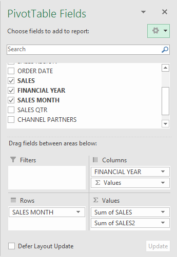
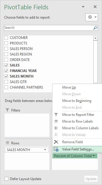
STEP 2: In the ROWS section put in the Sales Month field, in the COLUMNS put in the Financial Year field and in the VALUES area you need to put in the Sales field twice, I explain why below:
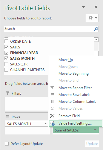
STEP 3: Click the second Sales field’s (Sum of SALES2) drop down and choose Value Field Settings
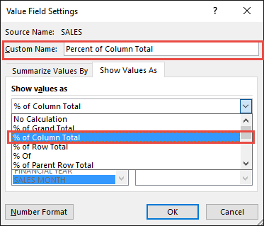
STEP 4: Select the Show Values As tab and from the drop down choose % of Column Total.
Also change the Custom Name into Percent of Column Total to make it more presentable. Click OK.
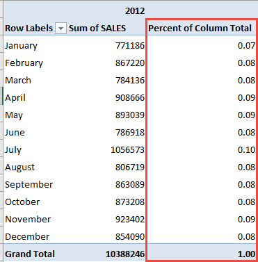
STEP 5: Notice that the Percent of Column Total data is in a decimal format that is hard to read:
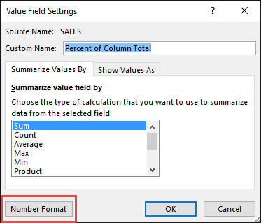
To format the Percent of Column Total column, click the second Sales field’s (Percent of Column Total) drop down and choose Value Field Settings.
The goal here is for us to transform numbers from a decimal format (i.e. 0.23), into a percentage format that is more readable (i.e. 23%).
STEP 6: Click the Number Format button.
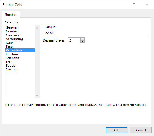
STEP 7: Inside the Format Cells dialog box, make your formatting changes within here and press OK twice.
In this example, we used the Percentage category to make our Percent of Column Total numbers become more readable.
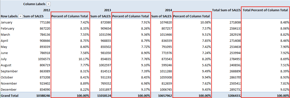
You now have your Pivot Table, showing the Percent of Column Total for the sales data of years 2012, 2013, and 2014.
All of the sales numbers are now represented as a Percentage of each column (Years 2012, 2013 and 2014), which you can see on each column is represented as 100% in totality:

Bryan
Bryan Hong is an IT Software Developer for more than 10 years and has the following certifications: Microsoft Certified Professional Developer (MCPD): Web Developer, Microsoft Certified Technology Specialist (MCTS): Windows Applications, Microsoft Certified Systems Engineer (MCSE) and Microsoft Certified Systems Administrator (MCSA).
He is also an Amazon #1 bestselling author of 4 Microsoft Excel books and a teacher of Microsoft Excel & Office at the MyExecelOnline Academy Online Course.


