Show The Percent of Parent Row Total With Excel Pivot Tables

Excel Pivot Tables have a lot of useful calculations under the SHOW VALUES AS option and one that can help you a lot is the PERCENT OF PARENT ROW TOTAL calculation. This is a new calculation in Excel 2010 and onwards. This option will immediately calculate the percentages for you from a table filled with numbers such as sales data, expenses, attendance, or anything that can be quantified.

Key Takeaways

• Add Context to Subcategories – Displaying percent of parent helps highlight how each item contributes to its category total.

• Use Value Field Settings Efficiently – Right-click a Pivot Table value → Show Values As → % of Parent Row Total to enable this feature.

• Ideal for Hierarchical Data – This is especially useful in data with multiple levels (e.g., Region → Country → City).

• Makes Comparisons Intuitive – Seeing percentages within categories helps identify strong or weak performers quickly.

• Works in Both Classic and Tabular Layouts – Percent of parent totals can be shown regardless of how the Pivot Table is displayed.

How to Show The Percent of Parent Row Total With Excel Pivot Tables

STEP 1: Insert a new Pivot table by clicking on your data and going to Insert > Pivot Table > New Worksheet or Existing Worksheet

 

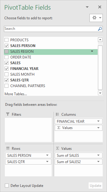
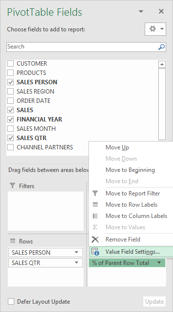
STEP 2: In the ROWS section put in the Sales Person and Sales Qtr fields, in the COLUMNS put in the Financial Year field and in the VALUES area you need to put in the Sales field twice, I explain why below:

 

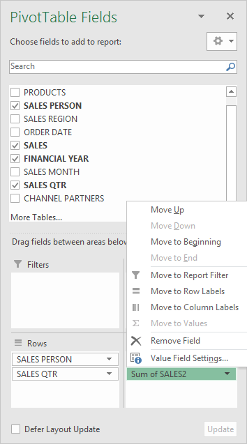
STEP 3: Click the second Sales field’s (Sum of SALES2) drop down and choose Value Field Settings

 

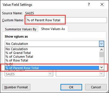
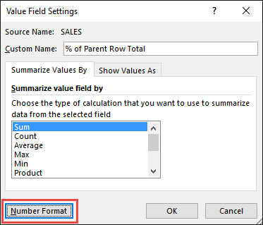
STEP 4: Select the Show Values As tab and from the drop down choose % of Parent Row Total. 

Also change the Custom Name into % of Parent Row Total to make it more presentable. Click OK.

 

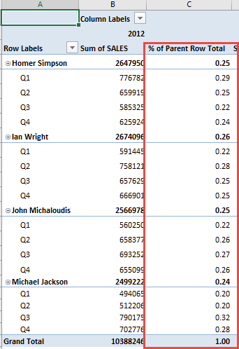
STEP 5: Notice that the % of Parent Row Total data is in a decimal format that is hard to read:

 

To format the % of Parent Row Total column, click the second Sales field’s (% of Parent Row Total) drop down and choose Value Field Settings. 

The goal here is for us to transform numbers from a decimal format (i.e. 0.23), into a percentage format that is more readable (i.e. 23%).

 

STEP 6: Click the Number Format button.

 

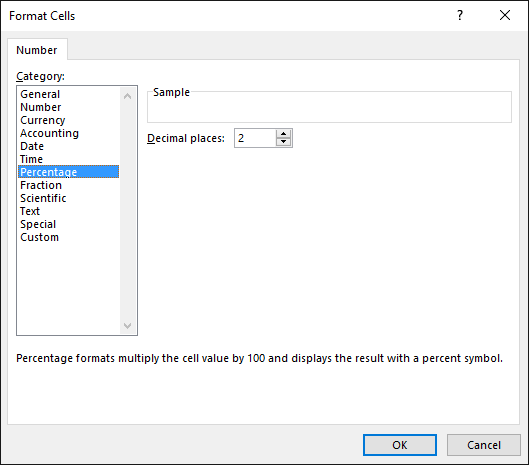
STEP 7: Inside the Format Cells dialog box, make your formatting changes within here and press OK twice.  

In this example, we used the Percentage category to make our % of Parent Row Total numbers become more readable.

 

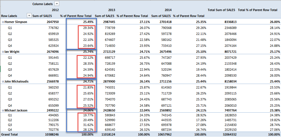
You now have your Pivot Table, showing the % of Parent Row Total for the sales data of years 2012, 2013, and 2014.

All of the sales numbers are now represented as a Percentage of its Parent’s subtotal.  

You can see that each red box is represented as 100% in totality for each encapsulating blue box i.e. Quarterly Sales as a percentage of each Sales Person´s Total Sales

Frequently Asked Questions

What is “Percent of Parent Row Total” in Pivot Tables?
It shows a value as a percentage of its immediate parent category, rather than the overall total.

How do I apply this setting in a Pivot Table?
Right-click the value field → choose “Show Values As” → select “% of Parent Row Total.”

Can I use this with multiple row levels in my Pivot Table?
Yes, it works best when you have hierarchical fields in the Row Labels section.

Does this option affect the actual data?
No, it only changes how the values are displayed; your underlying data remains unchanged.

Is it possible to show both raw values and percentages together?
Yes, just drag the same field twice into the Values area—one for the raw total, the other formatted as % of Parent Row Total.