Excel Pivot Tables have a lot of useful calculations under the SHOW VALUES AS option and one that can help you a lot is the Excel Pivot Table Percentage of Row Total. This option will immediately calculate the percentages for you from a table filled with numbers such as sales data, expenses, attendance, or anything that can be quantified.
Key Takeaways:
- Percent of Row Total Calculation: Excel Pivot Tables allow you to calculate percentages based on row totals by applying a “Show Values As” option. This is useful for comparing the contribution of each value to the total within a row.
- Easy to Apply: To show percentages, right-click on the value field in the Pivot Table, select Show Values As, and choose % of Row Total from the list. Excel will then display each data point as a percentage of its respective row total.
- Useful for Data Analysis: Displaying percentages of row totals helps in analyzing the relative contribution of each item or category within a specific row, which can be especially useful for sales data, performance analysis, and financial summaries.
- Dynamic Calculation: The percentage calculation is dynamic, meaning that as the data in the Pivot Table changes or filters are applied, the percentages automatically update, providing real-time insights.
- Flexible Formatting Options: Once the percentages are displayed, you can format the values to control decimal places, percentage symbols, and overall appearance, allowing for a more professional and readable report.
Table of Contents
How to Show The Percent of Row Total With Excel Pivot Tables
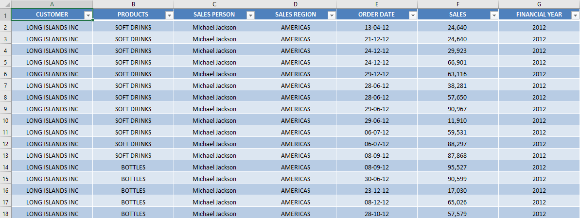
STEP 1: Select any cell in the Data Table
STEP 2: Go to Insert > PivotTable.
STEP 3: In the Create PivotTable dialog box, select table range and New Worksheet and then Click OK.
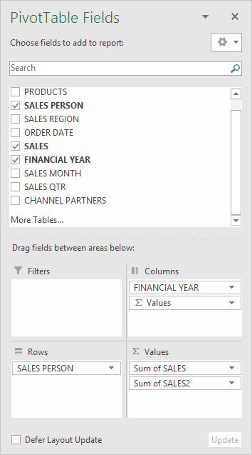
STEP 4: In the ROWS section put in the Sales Person field, in the COLUMNS put in the Financial Year field and in the VALUES area you need to put in the Sales field twice, I explain why below:
A Pivot Table will be created and looks like this:
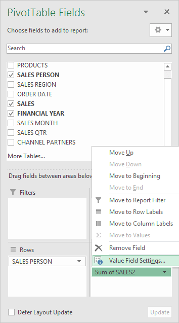
STEP 5:Click the second Sales field’s (Sum of SALES2) drop down and choose Value Field Settings
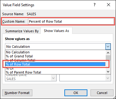
STEP 6: Select the Show Values As tab and from the drop down choose % of Row Total.
Also, change the Custom Name into Percent of Row Total to make it more presentable. Click OK.
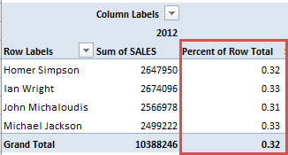
STEP 7: Notice that the Percent of Row Totaldata is in a decimal format that is hard to read:
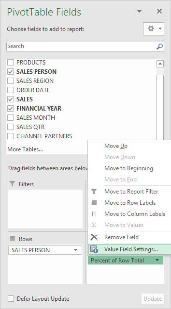
To format the Percent of Row Totalcolumn, click the second Sales field’s (Percent of Row Total) drop down and choose Value Field Settings.
The goal here is for us to transform numbers from a decimal format (i.e. 0.23), into a percentage format that is more readable (i.e. 23%).
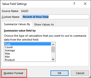
STEP 8: Click the Number Format button.
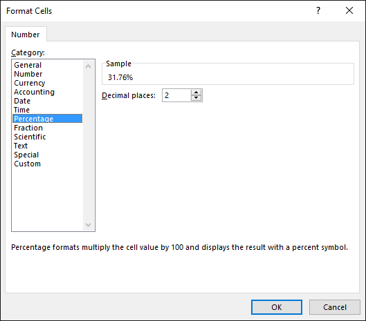
STEP 9: Inside the Format Cells dialog box, make your formatting changes within here and press OK twice.
In this example, we used the Percentage category to make our Percent of Row Total numbers become more readable.
You now have your Pivot Table, showing the Percent of Row Total for the sales data of years 2012, 2013, and 2014.
All of the sales numbers are now represented as a Percentage of each row (Years 2012, 2013 and 2014), which you can see on each row is represented as 100% in totality.
Particularly the yellow highlighted ones would total to 100% for the first row:
Frequently Asked Questions
How do I show the percentage of the row total in an Excel Pivot Table?
To display the percentage of row total, right-click on any value in the Values field of the Pivot Table, select Show Values As, and then choose % of Row Total. This will show each value as a percentage of its respective row total.
Can I apply this percentage calculation to multiple rows or columns?
Yes, you can apply the % of Row Total calculation to multiple rows or columns in your Pivot Table. Simply select the desired field in the Values section, right-click, and apply the calculation. Excel will calculate the percentage of row totals for all relevant rows or columns.
Does the percentage update automatically when I filter or change data in my Pivot Table?
Yes, the percentages are dynamic and will update automatically whenever you apply filters or change the data in the Pivot Table. The percentage calculations always reflect the current data displayed in the table.
Can I control the number of decimal places in the percentage values?
Yes, you can format the percentage values to control the number of decimal places. Right-click on the percentage values, select Number Format, and then choose Percentage with the desired number of decimal places.
Why does the percentage of row total add up to more than 100%?
The percentage of row total might add up to more than 100% if there are duplicate or overlapping data points in the Pivot Table. Check your data to ensure that each entry is unique, or consider adjusting your data set to remove any duplicates or inconsistencies.

Bryan
Bryan Hong is an IT Software Developer for more than 10 years and has the following certifications: Microsoft Certified Professional Developer (MCPD): Web Developer, Microsoft Certified Technology Specialist (MCTS): Windows Applications, Microsoft Certified Systems Engineer (MCSE) and Microsoft Certified Systems Administrator (MCSA).
He is also an Amazon #1 bestselling author of 4 Microsoft Excel books and a teacher of Microsoft Excel & Office at the MyExecelOnline Academy Online Course.
