5 Best Ways to Split String in Excel (Free Examples)

Many times, users are provided with unformatted and unclean data to work on.

It can be really difficult to apply filters, sort, or even create Pivot Tables using those unstructured data.

Microsoft Excel has a variety of functions and features that can be used to split those combined texts into separate columns and make data management more efficient.

In this article, we will be covering the 5 best ways to split string in Excel with our Free Step By Step Examples & Practice Workbook!

Let’s look at these methods thoroughly!

Download the Excel Workbook below to follow along and understand how to split string in Excel –

Download excel workbookSplit-String-in-Excel.xlsx

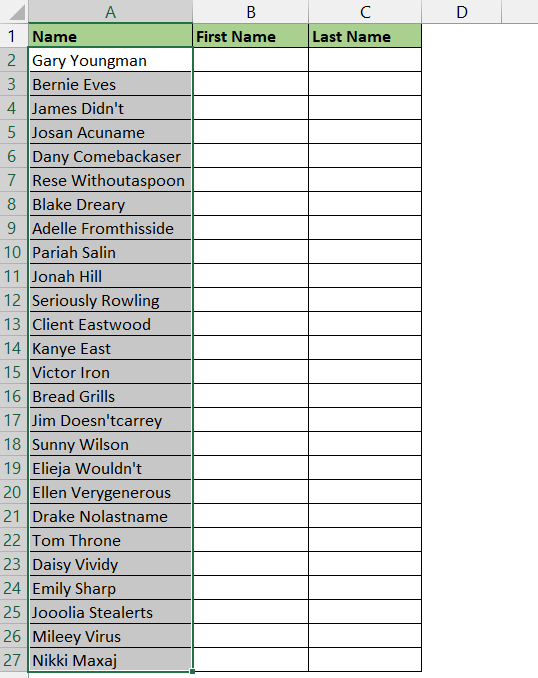
Ever encountered a situation where you have a data set of employee full names in one column and want to split them into separate columns? No worries. Excel has an excellent ad-hoc solution to this – Text to Column.

This feature allows you to split text into separate columns using a delimiter like a comma, space, semi-column, etc. Follow the steps below to know how to split string in Excel using Text to Columns –

STEP 1: Select the range containing the full names of the employees.

STEP 2: Go to Data > Text to Columns.

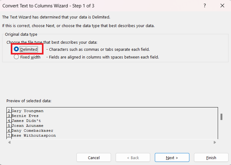
STEP 3: In the Convert Text to Columns dialog box, select Delimited > Next.

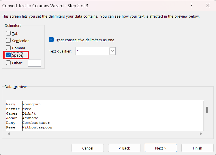
STEP 4: Select the delimiter for the data. Here, it is Space. Check the Data Preview at the bottom and then click Next.

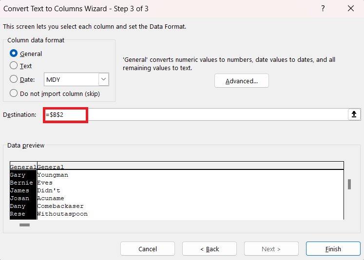
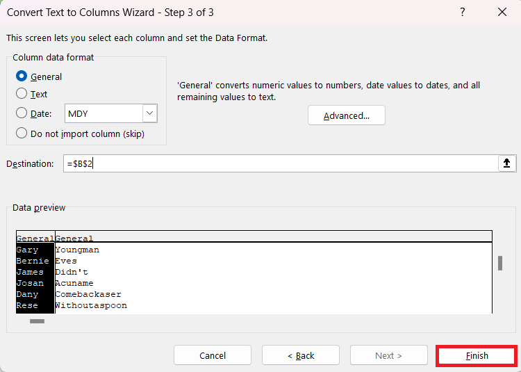
STEP 5: Select cell $B$2 as the destination and click Next.

STEP 6: Select Finish.

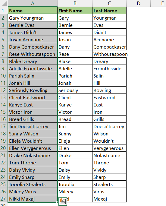
The full name of the employees are now separated into 2 columns – First name and Last name.

 

Method 2: LEFT, RIGHT & MID Function

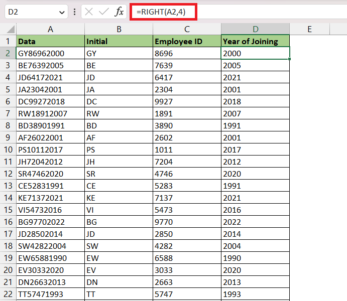
In this example, we have employee data in the following format – AL56442020

• AL – Employee’s initials
• 5644- Employee ID
• 2020- Year of joining

We can use LEFT, RIGHT, and MID functions to extract all three parts of this data. Follow the steps below to know how to split string in Excel –

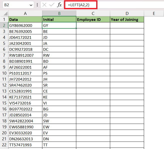
STEP 1: Enter the LEFT function. This function is used to extract the employee’s initial i.e. first 2 characters from the text.

=LEFT(A2,2)

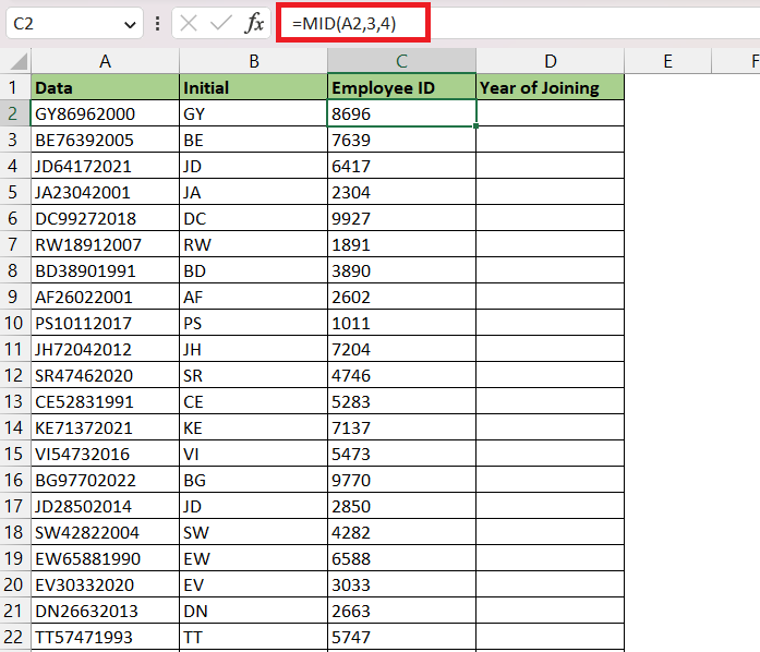
STEP 2: Enter the MID function. This function is used to extract the employee’s id i.e. 4 characters starting from the 3rd position of the text.

=MID(A2,3,4)

STEP 3: Enter the RIGHT function. This function is used to extract the employee’s year of joining i.e. 4 characters from the end of the text.

=RIGHT(A2,4)

 

Method 3: Text Functions

If you want to check where a specific text is located in the source text, it is very easy to search for the position using the FIND Formula!

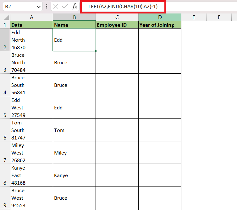
In this example, we have the first name and employee id, and year of joining separated by a line break. CHAR(10) in Excel is used to get a line break in a cell. We will be using the FIND function to get the position of the line break.

Follow the steps below to learn how to split string in Excel to get them in separate columns. –

STEP 1: Enter the following formula to get the first name i.e. all characters before the 1st instance of line break.

=LEFT(A2,FIND(CHAR(10),A2)-1)

• Here, the FIND function will provide you with the position of the 1st line break.
• We will subtract 1 because we do not need the line break in your result.
• The LEFT function will extract all characters left to this position.

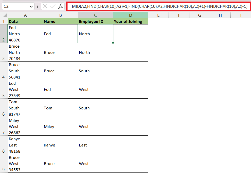
STEP 2: Enter the following formula to get the region i.e. all characters in between the 1st and 2nd line break.

=MID(A2,FIND(CHAR(10),A2)+1,FIND(CHAR(10),A2,FIND(CHAR(10),A2)+1)-FIND(CHAR(10),A2)-1)

Here, the MID function will provide the region. It has three arguments –

• text – It is the source text located in cell A2.
• start_num – It is the starting position for the MID function. This will be the position of 1st line break, plus 1 i.e. FIND(CHAR(10),A2) + 1.
• num_chars – It is the number of characters that need to be extracted. This will be the difference between the position of 2nd line break and 1st line break, minus 1 i.e. FIND(CHAR(10),A2,FIND(CHAR(10),A2)+1)-FIND(CHAR(10),A2)-1

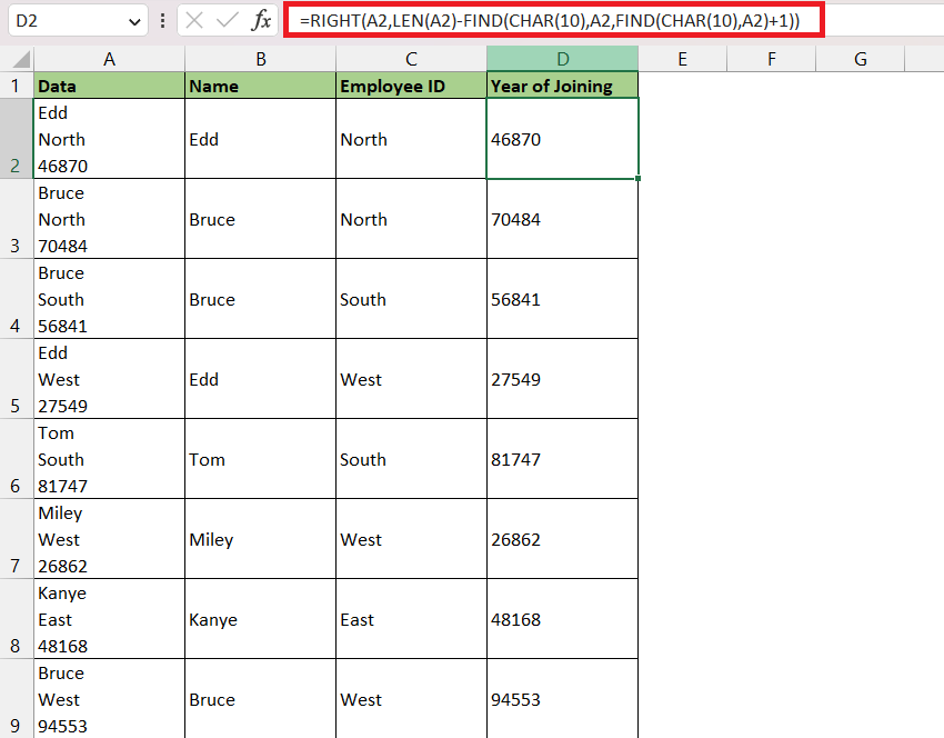
STEP 3: Enter the following formula to get the sales amount i.e. all characters after the 3rd line break.

=RIGHT(A2,LEN(A2)-FIND(CHAR(10),A2,FIND(CHAR(10),A2)+1))

Here, the RIGHT function will provide the region. It has three arguments –

• text – It is the source text located in cell A2.
• num_chars – It is the number of characters that need to be extracted. This will be the difference between the length of the text and position of 2nd line break, plus 1 i.e. LEN(A2)-FIND(CHAR(10),A2,FIND(CHAR(10),A2)+1

 

Method 4: TEXTSPLIT Function

TEXTSPLIT function can be used to split string in Excel by a given delimiter and display the result in multiple cells. It can split the text into both columns as well as rows. It is like a formula version of the Text-to-Column feature in Excel but it is much more versatile.

This function is exclusively available for Excel 365 subscribers.

The syntax of this function is –

=TEXTSPLIT(text, col_delimiter, [row_delimiter], [ignore_empty], [match_mode], [pad_with])

• text – The text you want to split. Required.
• col_delimiter – The text that marks the point where to spill the text across columns.
• row_delimiter – The text that marks the point where to spill the text down rows. Optional.
• ignore_empty – Specify TRUE to ignore consecutive delimiters. Defaults to FALSE, which creates an empty cell. Optional.
• match_mode – Specify 1 to perform a case-insensitive match. Defaults to 0, which does a case-sensitive match. Optional.
• pad_with – The value with which to pad the result. The default is #N/A.

In this example, let us see how to split string in Excel using the TEXTSPLIT function.

STEP 1: Enter the TEXTSPLIT formula –

=TEXTSPLIT

STEP 2: Enter the 1st argument i.e. text.

=TEXTSPLIT(B1,

STEP 3: Enter the 2nd argument i.e. col_delimiter. Here, it is left blank as we will split the text row-wise not column-wise.

=TEXTSPLIT(B1,,

STEP 4: Enter the 3rd argument i.e. row_delimiter. Here, it is CHAR(10).

=TEXTSPLIT(B1,,CHAR(10))

Repeat the same steps for the region and salary columns as well. The three rows will automatically be filled with the desired result!

 

Method 5: Flash Fill

Flash Fill in Excel is a feature that was introduced in Excel 2013. It is very handy as Excel predicts the rest of your inputs based on the first entry that you have placed. Once its prediction is correct and you confirm it, it will fill the rest of the rows literally in a flash!

The cool thing with Excel’s Flash Fill is there is no need to use formulas and removes manual repetitiveness, saving you heaps of time in the process!

Follow the steps below to understand how to use Flash Fill to split string in Excel –

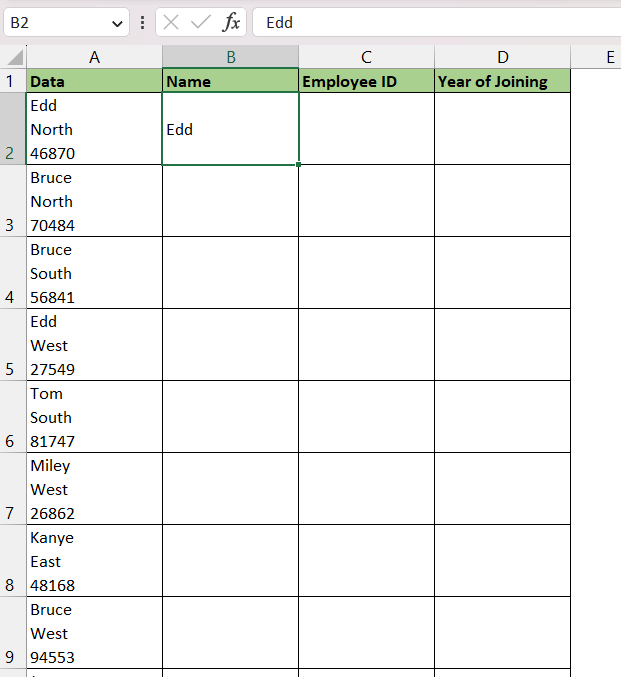
STEP 1: Type the first name in cell B2.

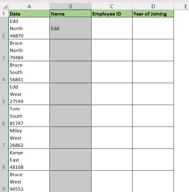
STEP 2: Select the range where you need the first names to be displayed. Here, it is B2:B27.

STEP 3: Go to Home > Fill > Flash Fill.

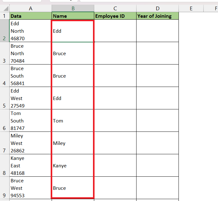
All the first names will be filled automatically.

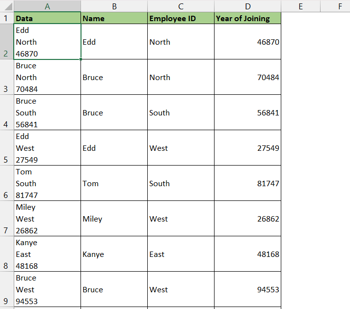
Repeat the steps for the region and salary columns as well. This will split string in Excel.