The Ultimate Guide to Excel Strikethrough Text

Excel Strikethrough is a formatting feature that allows you to draw a line through text or numbers within a cell. This is useful for indicating that certain tasks are completed or that they are no longer relevant. In this article, we will cover different ways to apply strikethrough in Microsoft Excel.

Key Takeaways:

• Strikethrough helps in visually marking completed or irrelevant items.
• It aims at better data management and historical tracking.
• Apply Strikethrough quickly using keyboard shortcuts – Ctrl + 5.
• Customize your Excel Ribbon to include a Strikethrough button for easy access.
• Use conditional formatting to automate Strikethrough based on specific criteria.

 

What Is Excel Strikethrough?

Excel Strikethrough is like your virtual highlighter, but instead of making things stand out, it helps you indicate the completion or irrelevance of tasks and items directly onto your data sheet. Imagine having a to-do list and drawing a line through each item you’ve completed – that’s exactly what the Strikethrough feature does to your text or numbers in Excel cells.

 

How to Strikethrough in Excel

Method 1: Keyboard Shortcuts

STEP 1: Select the cell you want to strikethrough.

STEP 2: Now, hold ‘CTRL+5‘. You will then see a strikethrough in the selected cell ‘A2‘.

Mac users, on the other hand, should use the Command + Shift + X combo.

Method 2: Ribbon Customization

STEP 1: Right-click anywhere on the Ribbon and choose ‘Customize the Ribbon’.

STEP 2: Choose the ‘Home’ tab and click ‘New Group’ to create a custom group.

STEP 3: Name your group.

STEP 4: With your new group selected, choose ‘Commands Not in the Ribbon’ from the drop-down menu.

STEP 5: Scroll to find ‘Strikethrough,’ select it, and click ‘Add.’

STEP 6: Hit ‘OK’. Your Strikethrough button is ready for action on the Ribbon.

Now, Strikethrough tool is just a click away.

 

Manual versus Automatic

Manual Application

STEP 1: Start by selecting the cell or range where you want to apply Strikethrough.

STEP 2: Right-click the selection and select ‘Format Cells’ from the context menu.

STEP 3: In the ‘Format Cells’ dialog box, go to the ‘Font’ tab.

STEP 4: Look for the Strikethrough checkbox and click on it to mark it.

STEP 5: Finish by clicking ‘OK,’ and you will see the Strikethrough effect applied to your selection.

This manual method gives you the control to apply this format to specific items.

Automatic Strikethrough

STEP 1: First, select the range of cells you wish to apply automatic Strikethrough to.

STEP 2: Go to the ‘Home’ tab and locate ‘Conditional Formatting’ in the ‘Styles’ group. Click it and select ‘New Rule.’

STEP 3: In the ‘New Formatting Rule’ dialog, choose ‘Use a formula to determine which cells to format.’

STEP 4: Enter the condition formula in the box that reads “Format values where this formula is true.” For example, typing =B3="Completed" will apply Strikethrough to any cell in your selected range that contains the word “done.” After setting the formula, click ‘Format’.

STEP 5: Now move to the ‘Font’ tab, and choose ‘Strikethrough.’ Confirm all your actions with ‘OK,’ and watch as cells automatically get struck through when they meet the conditions you specified.

STEP 6: Now you can preview the strikethrough formatting selected by you, then click “OK”.

Automatic Strikethrough ensures your spreadsheet remains up-to-date with minimal manual intervention.

 

Tips & Tricks

Partial Strikethroughs

STEP 1: Double-click the cell to enable editing mode or press F2 after selecting the cell.

STEP 2: Highlight only the portion of text you want to strike through by dragging your mouse over it or using the Shift + arrow keys.

STEP 3: With the text selected, either right-click and choose ‘Format Cells’ or use the familiar shortcut; ‘Ctrl + 1’.

STEP 4: In the ‘Format Cells’ dialog box, tick the ‘Strikethrough’ checkbox under the ‘Font’ tab & Click ‘OK’.

RESULT: You will see that only the selected part of the text has the Strikethrough effect.

Use Format Painter

To replicate Strikethrough formatting across different parts of your spreadsheet, the Format Painter tool can be used.

STEP 1: Select the cell that has the Strikethrough format you want to copy.

STEP 2: Click the ‘Format Painter’ icon in the ‘Home’ tab (it looks like a paintbrush).

STEP 3: Then, simply select the cells where you’d like to apply the same formatting.

 

Remove Strikethrough

Manual Application

STEP 1: Click on the cell or select the range where you want to remove Strikethrough.

STEP 2: Press Ctrl + 1 to open the ‘Format Cells’ dialog box, or right-click and choose ‘Format Cells’ from the context menu.

STEP 3: Under the ‘Font’ tab, uncheck Strikethrough. Click OK.

The Strikethrough formatting will be removed.

Automatic Application

STEP 1: Go to the Home tab.

STEP 2: Select Conditional Formatting > Manage Rules.

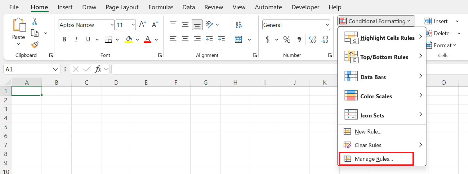
STEP 3: Delete the rule of Strikethrough.

It will be removed.

 

FAQs

How to do strikethrough text in Excel?

To do strikethrough text in Excel,

• Select the cells you want to format
• Use keyboard shortcut Ctrl + 5

What is the shortcut for strikethrough text?

The shortcut for applying strikethrough text in Excel is Ctrl + 5 on a Windows computer and Command + Shift + X on a Mac.

Can Strikethrough Be Sorted or Filtered within Excel?

Strikethrough itself cannot be directly used as a criterion for sorting or filtering in Excel.

Are There Any Strikethrough Accessibility Features for Excel Online Users?

Excel Online users have access to most of the standard accessibility features, including strikethrough formatting.

Where is the font strikethrough option?

In Excel, the strikethrough option is found in the ‘Font’ group under the ‘Home’ tab.