The Ultimate Guide to Total a Column in Excel

Calculating the total of a column is one of the most frequent and useful actions in Excel. Whether you are managing budgets, analyzing sales data, or tracking project hours, knowing how to sum a column accurately is a must-have skill. This guide will walk you through several methods to total a column in Excel, from the classic AutoSum to more advanced options like Power Query and VBA. Each method includes step-by-step instructions, common issues to avoid, and bonus tips to help you work smarter in Excel.

Key Takeaways

• The SUM function is the fastest way to total a column in Excel.
• AutoSum automatically detects ranges and inserts the SUM formula with a single click.
• Table Totals Row offers a quick way to sum columns within formatted tables.
• Power Query and VBA are powerful for automating or working with complex totals.
• Be cautious about hidden rows, filtered data, or blank cells when totaling columns.

Quick and Easy Methods to Total a Column

Harnessing the Power of AutoSum

AutoSum is one of the quickest ways to add up a column in Excel. By automatically summing contiguous numbers, it saves you time and effort. To use AutoSum, click on the cell below the column you want to total, and then click the “AutoSum” button on the toolbar. Excel will select the range it thinks you want to add, allowing you to adjust if necessary, and press “Enter” to get your result.

Exploring the SUM Function for Accuracy

The SUM function offers flexibility and precision, especially when you need to specifically define which cells to add. To use the SUM function, select a cell where you want the total to appear, type =SUM(, then choose the cells or range you wish to sum. Close the formula with a closing parenthesis ), and press “Enter”. This function is particularly useful if your data isn’t contiguous, allowing you to select discrete cells instead of an entire block. The formula looks like this: =SUM(A1:A10, C1:C5), where A1:A10 and C1:C5 are the ranges or cells being added.

Step-by-Step: How to Total a Column in Excel

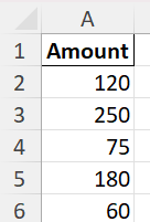
Step 1: Prepare Your Data

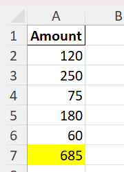
Start with your data in a clean column, for example:

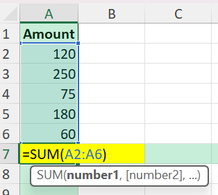
Step 2: Using the SUM Function

Click in a cell below your column (for example, A7) and enter:

=SUM(A2:A6)

This formula adds up all numbers in cells A2 through A6.

Step 3: Using AutoSum

Select the first empty cell below your column of numbers.
Click the AutoSum button on the Home tab (Σ icon).

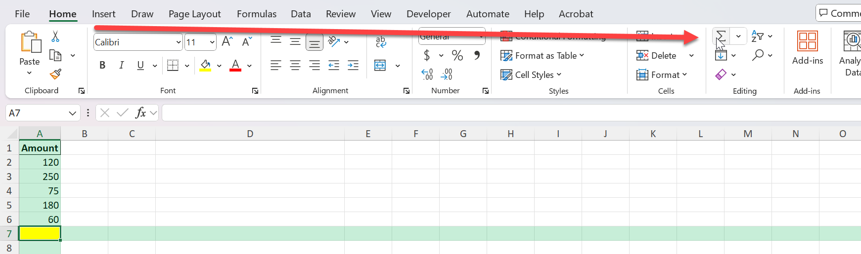
Press Enter.

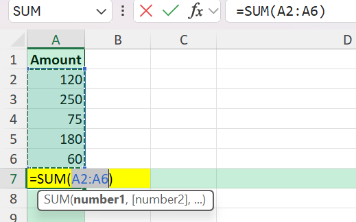
Excel will automatically create a SUM formula for your data range.

Common Mistakes or Tips

Blank Cells: SUM ignores blanks, but check if you expect a zero value.

Hidden/Filtered Rows: SUM includes hidden rows. Use SUBTOTAL for filtered data: =SUBTOTAL(9, A2:A100).

Mixed Data Types: Text in your column will be ignored. Make sure all data are numbers.

Cell References: Double-check your SUM range. Expanding data? Consider using Excel Tables so your totals update automatically.

Formula Placement: Place the total cell outside your data range to avoid circular references.

Bonus Tips & Advanced Scenarios

Summing Only Visible (Filtered) Rows:
Use SUBTOTAL to total only the rows visible after filtering.
=SUBTOTAL(9, A2:A100)

Using VBA to Sum a Column:
For automation, try this VBA macro:

Sub SumColumnA()
    Range("A8").Value = WorksheetFunction.Sum(Range("A2:A6"))
End Sub

This will place the sum in A8.

Dynamic Ranges with Structured References:
If your data is in a Table named “Table1”, use:
=SUM(Table1[Amount])

Use Cases for Totaling Columns in Excel

Summing sales amounts for monthly or quarterly reporting

Calculating total project costs from itemized expenses

Adding up student scores or attendance in a class roster

Summing inventory counts for stock management

Automating batch processing of totals across multiple sheets

Advanced Techniques for Precise Totals

Using SUMIF to Meet Conditions

The SUMIF function is ideal when you need to add data that meets specific criteria. It allows you to perform conditional sums based on characteristics like text criteria, numeric values, or dates. For instance, if you’d like to add only the sales figures that exceed $1,000, you use the formula =SUMIF(range, criteria, sum_range). Here’s an example: =SUMIF(B2:B10, ">1000", C2:C10), where B2:B10 is the range for criteria evaluation, “>1000” is the condition, and C2:C10 is where the actual numbers to sum are located.

This method is especially powerful when dealing with large data sets, as it streamlines the process of extracting relevant data.

Leveraging Subtotal for Filtered Data

The Subtotal function is perfect for totaling data that you’ve filtered within a spreadsheet. Unlike the SUM function, Subtotal dynamically recalculates totals based on the visible rows, ignoring any that are hidden by filters. To use it, place your cursor in an empty cell, select from the menu: “Data” > “Subtotal”. Alternatively, use the formula: =SUBTOTAL(function_num, range), with function_num as the type of calculation (e.g., 9 for SUM) and range as the dataset. For example, =SUBTOTAL(9, A2:A10) adds only visible cells in the A2:A10 range.

Frequently Asked Questions (FAQ)

Can I total multiple columns at once?
Yes. Use =SUM(A2:A6, B2:B6) or apply SUM to each column as needed.

What if my data expands?
Use Excel Tables. Totals update automatically as new data is added.

How do I avoid totaling hidden rows?
Use SUBTOTAL for filtered data: =SUBTOTAL(9, A2:A100)

What’s the quickest shortcut to total a column?
Select the first empty cell below your column and press Alt + =.

Can I sum only numbers with a specific condition?
Yes, use SUMIF or SUMIFS for conditional summing. Example: =SUMIF(B2:B6, "Approved", A2:A6)