Split Screen feature allows you to simultaneously view and edit different sections of the worksheet. This function is important for maintaining focus on various data points without losing your place. In this article, you will learn how to split the screen in Excel.
Key Takeaways
- Split Screen allows you to view different parts of a worksheet at once.
- It reduces the need for constant scrolling or switching tabs.
- This feature simplifies the comparison of disparate data sets.
- Excel allows vertical, horizontal, or combined splits.
- Each pane operates independently.
Table of Contents
Introduction to Split Screen
What Is Split Screen?
Imagine a scenario where you need to compare your monthly sales from two different quarters that are several rows apart. Without split screen, you will have to scroll back and forth and may lose track of the data.
Split screen in Excel allows you to divide your workbook into separate panes. Each pane can independently scroll through different areas of your data. You can view and edit multiple sections of your spreadsheet simultaneously.
Advantages of Split Screen
The benefits of using split screen are:
- You can compare different parts of the worksheet easily.
- It allows you to keep headers and labels visible.
- It allows you to analyze a large dataset quickly.
- It can improve your productivity.
- It reduces the need for excessive scrolling.
How to Split Screen
Follow these simple steps to split the screen:
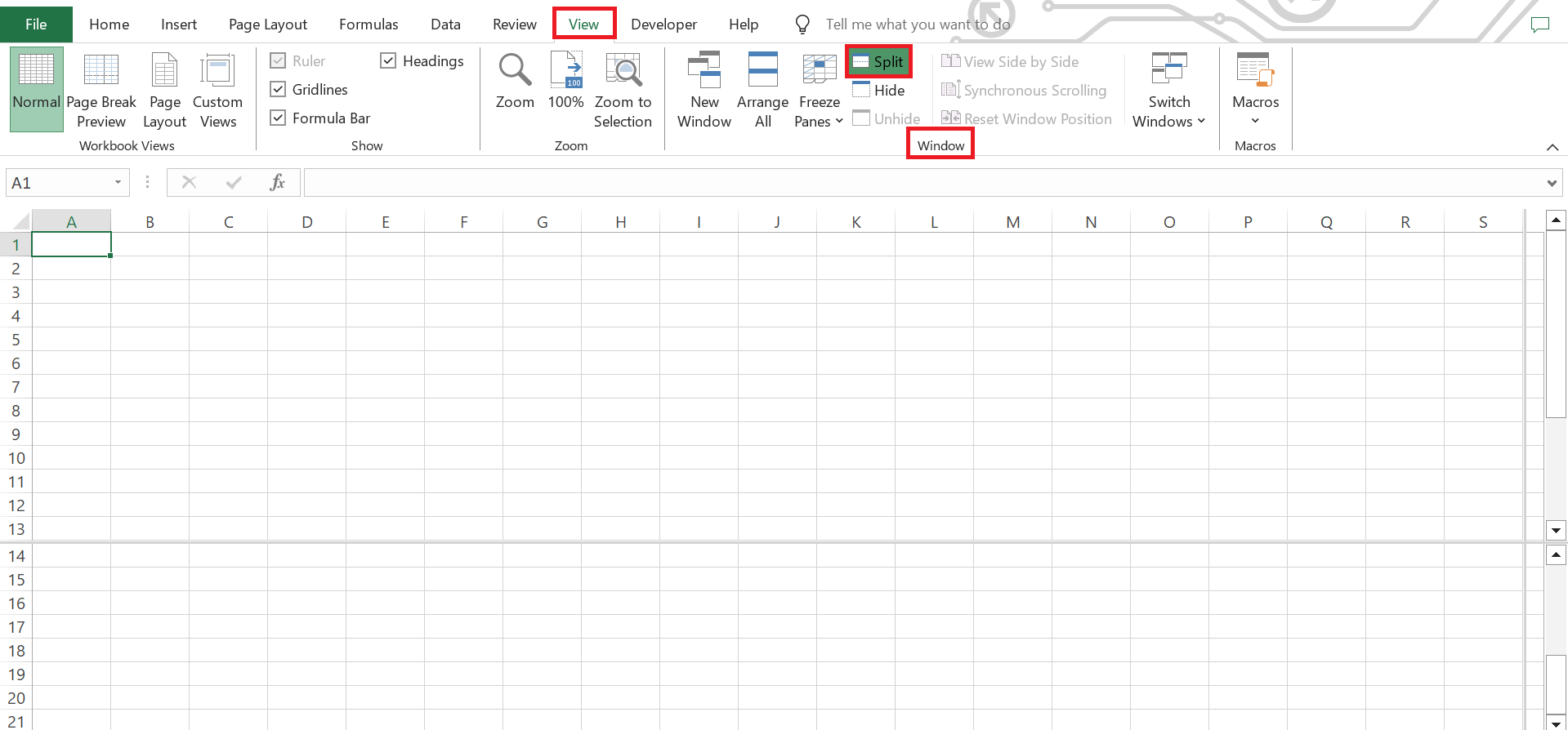
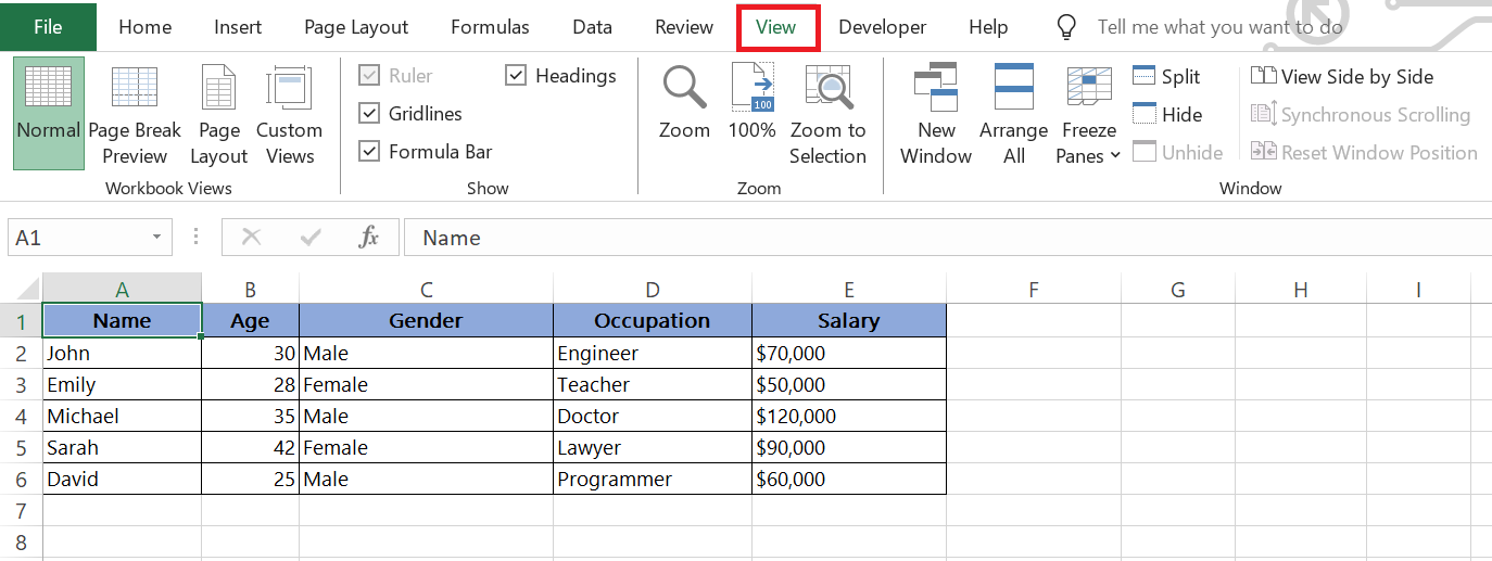
STEP 1: Click on the View tab.
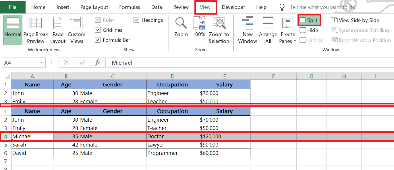
STEP 2: In the Window group, click on Split.
Your screen will divide into two or four panes depending on where you position your cursor.
You decide whether to split your window vertically, horizontally, or both ways by placing the cursor accordingly before clicking “Split.”
Advanced Techniques
Horizontal Split
STEP 1: Go to the “View” tab and in the “Window” group,
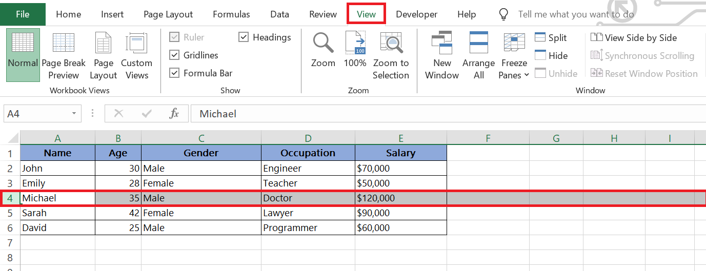
STEP 2: Select the row below where you want the split to occur.
STEP 3: Click on “Split.” This divides the data from the selected row, and two screens are created. It helps in analyzing each variable side by side.
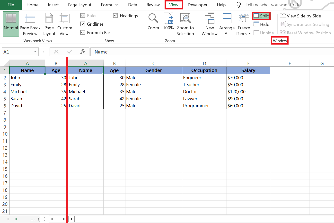
Vertical Split
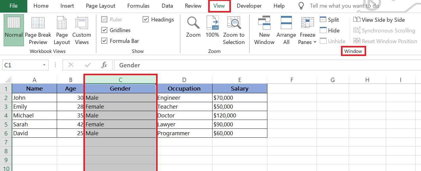
STEP 1: Go to the “View” tab and in the “Window” group,
STEP 2: Select the column beside where you want the split to occur
STEP 3: Click on “Split.” This divides the data from the selected column into two screens which helps in making comparison.
Both Horizontal and Vertical Split
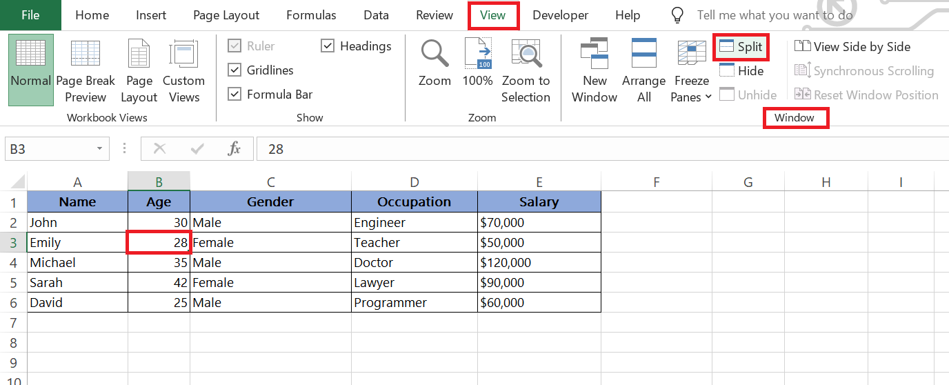
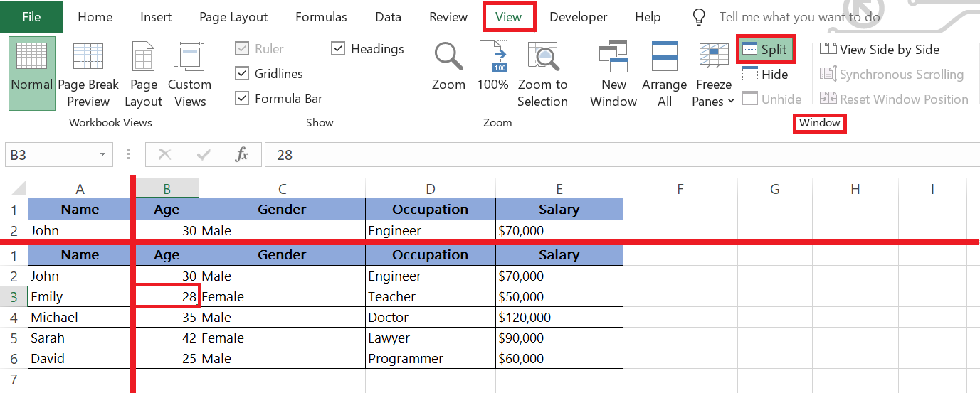
STEP 1: Click on a cell that is not in the first column or row.
STEP 2: Choose “Split” from the “View” tab as before.
Don’t worry if you need to adjust after applying the split—you can click and drag the split lines to fine-tune the size of each pane until it fits your needs just right.
Scroll Simultaneously
After the split screen, each pane operates independently. When you scroll in one pane, it does not affect the other pane.
However, you can also scroll panes simultaneously. This is useful when you want to compare data side by side. Follow the steps below for Synchronous Scrolling:
- Go to the View tab
- Click on Synchronous Scrolling
FAQs
How to split my Excel Windows?
To split your Excel window into two screens, follow the steps below:
- Select the cell where you want the split to appear
- Go to the View tab
- Click the Split button in the Window group.
Your window will split into two parts, either above and below or left and right of the selected cell.
How to use Excel split screen vertically?
To split your Excel screen vertically, choose a cell in the top row of the section you want to see on the right side of the split. Then, head to the “View” tab, look for the “Window” group, and click on “Split.” This will divide your screen so you have vertical panes side by side.
How to use Excel split screen both horizontally and vertically?
To split your Excel screen both horizontally and vertically, click on a cell that is below and to the right of where you want the splits to intersect. Next, navigate to the “View” tab, find the “Window” group, and click on “Split.” You’ll now have four separate panes that you can scroll through independently.
Can You Save an Excel Layout with Split Screen Presets?
Yes, in Excel, you can save a layout with split screen presets using the Custom Views feature. Go to the “View” tab, click “Custom Views,” then “Add” to name and save your current layout, including any split screen settings. This allows you to quickly switch to this layout in the future.
How to Split Screen Between Two Worksheets Effectively?
To split the screen between two worksheets effectively, open both worksheets in separate windows. Click “View” then “New Window” to create a new view of your active worksheet. Arrange the windows side by side by clicking “View” then “Arrange All” and select “Vertical.” Now you can view and work on both worksheets simultaneously
John Michaloudis is a former accountant and finance analyst at General Electric, a Microsoft MVP since 2020, an Amazon #1 bestselling author of 4 Microsoft Excel books and teacher of Microsoft Excel & Office over at his flagship MyExcelOnline Academy Online Course.


