Power Query is a free add-in created by Microsoft for Excel 2010 (or later) and you can download and install it for Excel 2010 and 2013:
Click to see tutorial on how to install Power Query in Excel 2013
Click to see tutorial on how to install Power Query in Excel 2010
In Excel 2016 it comes built in the Ribbon menu under the Data tab and within the Get & Transform group.
Power Query allows you to extract data from any source, clean and transform the data and then load it to another sheet within Excel, Power Pivot or the Power BI Designer canvas.
One of the best features is to Unpivot Columns.
What that does is transforms columns with similar characteristics (e.g. Jan, Feb, March…) and puts them in a unique column or tabular format (e.g. Month), which then allows you to do further analysis using Pivot Tables which was not possible before unpivoting.
Here is how this is done:
Download excel workbookUnpivot.xlsx
STEP 1: Highlight your data and go to Power Query > From Table > OK
STEP 2: This opens the Power Query editor and from here you need to select the columns that you want to unpivot
STEP 3: You then need to go to the Transform tab and select Unpivot Columns
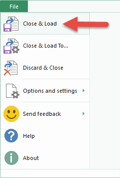
STEP 4: Go to the File tab and choose Close & Load
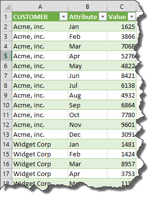
STEP 5: This will load and open the unpivoted data into a new worksheet with your Excel workbook. Now you can go crazy with your super analytical work, using Pivot Tables etc
THIS POST WAS INSPIRED BY THE FOLLOWING PODCAST SHOW:
John Michaloudis is a former accountant and finance analyst at General Electric, a Microsoft MVP since 2020, an Amazon #1 bestselling author of 4 Microsoft Excel books and teacher of Microsoft Excel & Office over at his flagship MyExcelOnline Academy Online Course.


