Varp in Excel Pivot Tables

Let us explore how to get Varp in Pivot Table, this shows the variability from the average or mean value of the group.

Exercise Workbook:

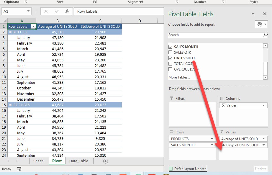
STEP 1: Here is our Pivot Table. Drag UNITS SOLD to the Values Area

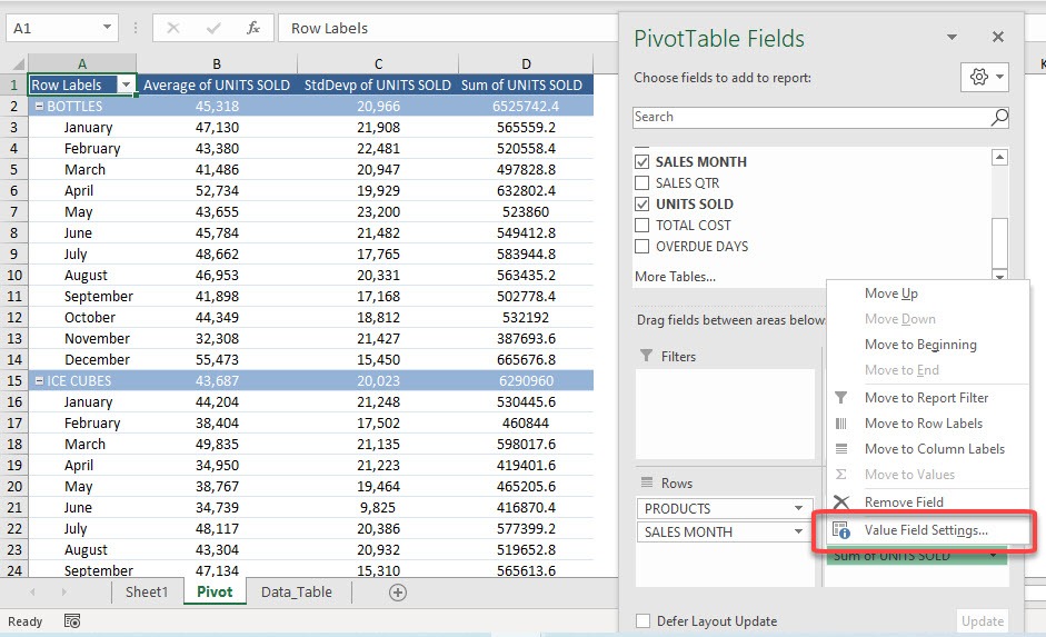
STEP 2: This will default to Sum of UNITS SOLD. Let us change that by clicking on the arrow and selecting Value Field Settings

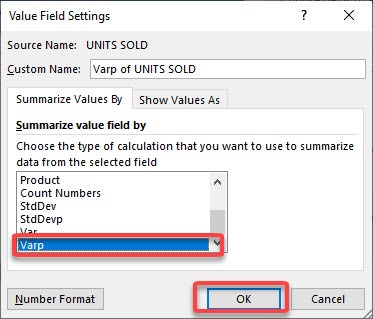
STEP 3: Select Varp and click OK.

We will use the Varp function as we have the complete data (population) used in the calculation. When only a portion of the data is used, then Var should be used instead.

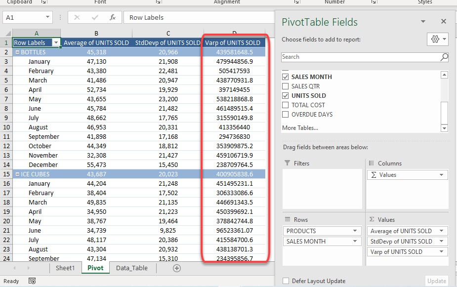
Now you have your Variance.

Did you know that the square root of the variance will give you the standard deviation value? Click here to learn how!

Make sure to download our FREE PDF on the 333 Excel keyboard Shortcuts here:

Bryan

Bryan Hong is an IT Software Developer for more than 10 years and has the following certifications: Microsoft Certified Professional Developer (MCPD): Web Developer, Microsoft Certified Technology Specialist (MCTS): Windows Applications, Microsoft Certified Systems Engineer (MCSE) and Microsoft Certified Systems Administrator (MCSA).

He is also an Amazon #1 bestselling author of 4 Microsoft Excel books and a teacher of Microsoft Excel & Office at the MyExecelOnline Academy Online Course.