Conditional Format a Cell´s Value

Microsoft Excel is more than just rows and columns filled with numbers and text. It is a powerhouse tool for data analysis, visualization, and decision-making. One of Excel’s most underrated yet highly effective features is Conditional Formatting. This feature allows you to highlight or format cells based on their values or specific criteria. By using Conditional Formatting, you can quickly spot trends, identify outliers, and make your data more visually appealing.

In this article, we’ll focus on Conditional Formatting a cell’s value—how to set it up, customize it, and make it interactive with dynamic references. By the end, you’ll be able to visually interpret your Excel data more effectively, whether you’re working with standard tables, Excel Tables, or Pivot Tables.

Key Takeaways:

• Conditional Formatting highlights cells automatically based on specific criteria, making trends and outliers easy to spot.
• It works in standard tables, Excel Tables, and Pivot Tables, adapting dynamically to your data.
• Using cell references for rules makes Conditional Formatting interactive and responsive to changes.
• Avoid excessive colors or formatting styles to keep your data clear and easy to interpret.
• Conditional Formatting is more efficient than manual formatting, especially for large datasets or dashboards.

 

The Importance of Conditional Formatting

What Is Conditional Formatting?

Conditional Formatting is a feature in Excel that applies formatting to cells automatically if they meet certain conditions. For example, you might want to highlight sales figures that exceed a certain threshold, mark negative numbers in red, or emphasize top-performing employees in a dataset.

The true power of Conditional Formatting is that it updates automatically when the underlying data changes. This makes it ideal for dashboards, reports, and dynamic data analysis.

Why Conditional Formatting Matters

Imagine you are tracking monthly sales across multiple regions. A table filled with raw numbers can be overwhelming. However, if you apply Conditional Formatting to highlight:

• Sales greater than a target number
• Months where revenue dropped below average
• Top 10% performers

…you immediately gain insights without manually scanning through the data.

In essence, Conditional Formatting turns numbers into visual cues, making it easier to analyze trends, compare data, and make informed decisions.

 

Step-by-Step Guide: Conditional Formatting a Cell’s Value

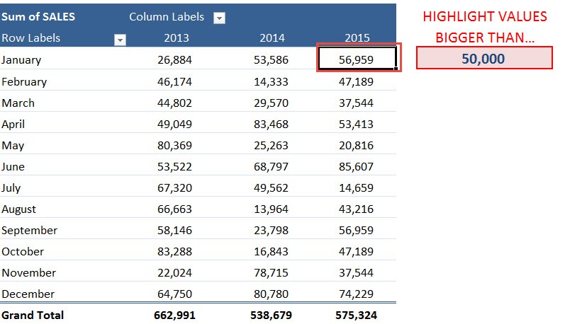
STEP 1: Select a cell in your Pivot Table.

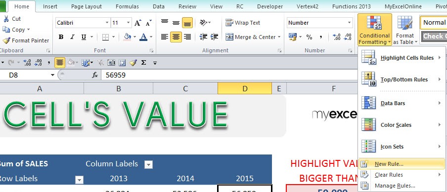
STEP 2: Go to Home > Conditional Formatting > New Rule

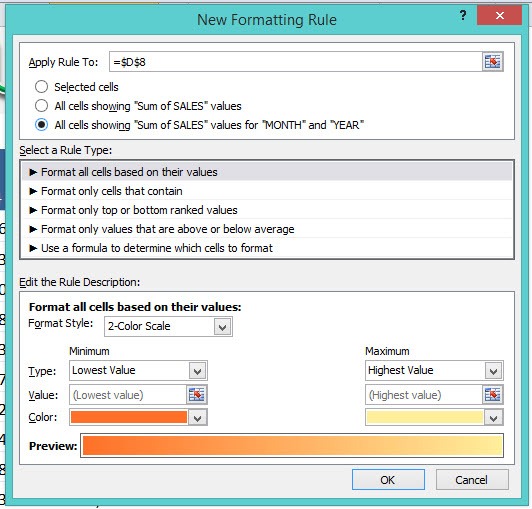
STEP 3: Set Apply Rule to the third option: All cells showing “Sum of SALES” values for “MONTH” and “YEAR”

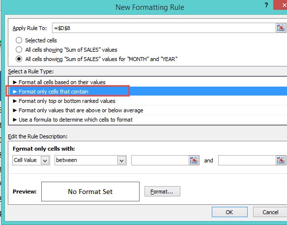
STEP 4: Select a rule type: Format Only Cells That Contain

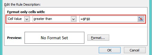
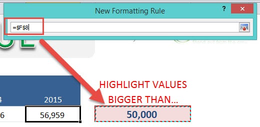
STEP 5: Edit the Rule Description. Go to Cell Value > Greater Than > Select The Cell

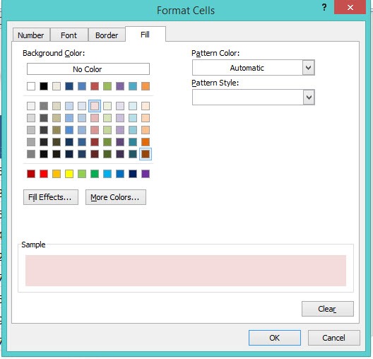
STEP 6: Select the cell format. Click Format and select a color. Click OK.

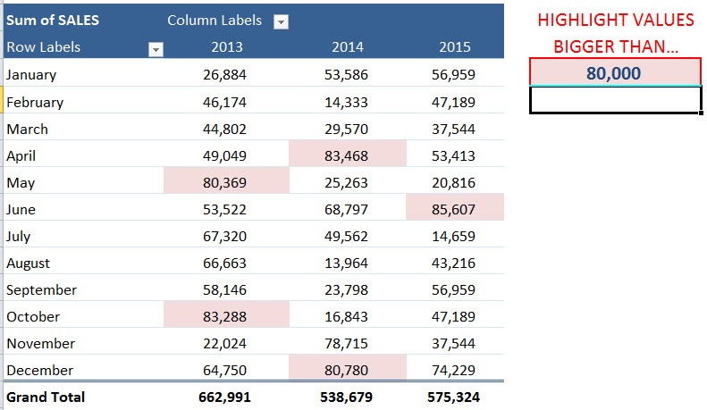
Try it out now! The highlight now happens dynamically when you update the value.

 

Best Practices for Using Conditional Formatting

Tips & Tricks

• Use Cell References for Dynamic Rules: Instead of hardcoding values, reference cells so the formatting updates dynamically.
• Avoid Excessive Formatting: Too many colors or styles can make your data confusing. Stick to 2–3 formatting styles.
• Leverage Built-In Rules: Excel provides “Top/Bottom Rules,” “Data Bars,” “Color Scales,” and “Icon Sets” for quick visualizations.
• Clear Rules Carefully: If a Conditional Formatting rule is no longer needed, clear it from the selected cells, table, or entire sheet.
• Combine Rules Strategically: You can apply multiple rules to the same cell range, but be mindful of priority—Excel applies rules in order of priority.

Conditional Formatting vs. Manual Formatting

Manual formatting (changing cell colors or fonts individually) may work for small datasets, but it becomes impractical for large tables. Conditional Formatting automates this process and ensures consistency, especially when the underlying data changes frequently. This is crucial in reports, dashboards, and live data analysis scenarios.

 

Practical Examples of Conditional Formatting a Cell’s Value

Here are some real-world examples of how you can apply Conditional Formatting effectively:

• Highlight High Sales: Format cells greater than your monthly target.
• Flag Low Inventory: Highlight products with stock below a critical level.
• Spot Negative Numbers: Automatically color negative balances in red.
• Performance Metrics: Highlight employees with above-average performance.
• Dynamic Thresholds: Reference a cell for a variable target, making your analysis interactive.

 

FAQs

1. What is Conditional Formatting in Excel?

Conditional Formatting is a feature that automatically applies formatting—such as colors, fonts, or borders—to cells that meet specific conditions. For example, you can highlight sales above a certain number or flag negative values. It updates dynamically when the underlying data changes. This makes it ideal for reports, dashboards, and analysis. It is a key tool for turning raw data into visual insights.

2. Why should I use Conditional Formatting instead of manual formatting?

Manual formatting can work for small datasets, but it is time-consuming and inconsistent for large tables. Conditional Formatting applies rules automatically across ranges or entire Pivot Tables. When your data changes, the formatting updates without extra effort. This ensures efficiency, consistency, and accuracy. It is especially useful for dashboards and recurring reports.

3. Can Conditional Formatting be dynamic based on another cell’s value?

Yes, by referencing another cell in your formatting rule, you can make it dynamic. For example, you can highlight all sales above the value in a reference cell. When the reference cell changes, the formatting updates automatically. This allows for interactive “what-if” scenarios. It makes your dashboards and analyses more flexible.

4. What are some practical examples of Conditional Formatting?

You can highlight high sales figures, flag low inventory, mark negative balances in red, or emphasize top-performing employees. Another example is setting dynamic thresholds where the target is referenced from another cell. This makes your data interactive and visually intuitive. Conditional Formatting can also use data bars, color scales, and icon sets. These examples help quickly identify important trends and anomalies.

5. How can I manage multiple Conditional Formatting rules effectively?

You can combine multiple rules on the same range, but order matters because Excel applies rules by priority. Always clear rules that are no longer needed to avoid conflicts. Stick to 2–3 formatting styles for clarity. Use built-in rules like Top/Bottom, Data Bars, or Color Scales for efficiency. Managing rules strategically ensures your data remains visually clear and accurate.