Let’s say you are in charge of a task to create a system where you have to randomly select customers for a special promotion in your small business. You want to ensure fairness and equal opportunity, giving every customer a chance to participate. But how do you go about selecting customers randomly?
Excel can make the selection process for the promotion unbiased and efficient. In this article, we will explore the methods that will allow you to Generate Random Numbers easily:
Let’s look at these methods thoroughly!
Download the Excel Workbook below to follow along and understand How to Use Substrings in Microsoft Excel
download excel workbookRandom-Numbers.xlsx
RAND Function: Generating Random Numbers Between 0 and 1
We want to randomly select customers from your customer database.
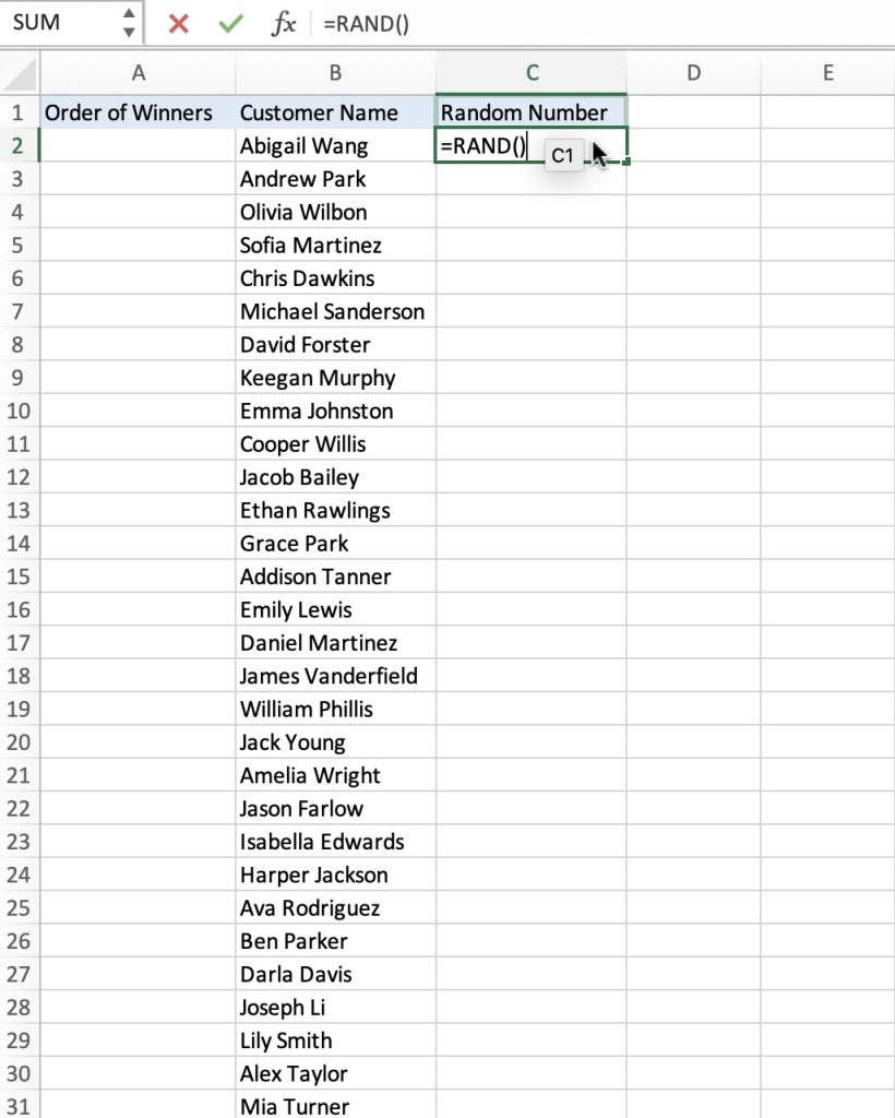
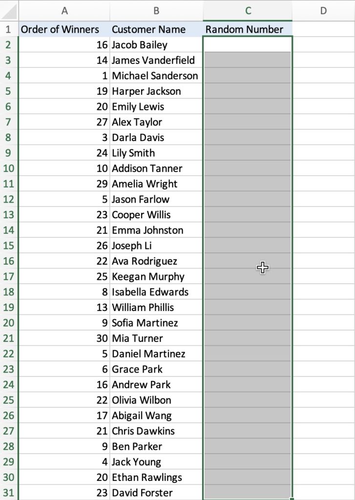
Open an Excel worksheet and create a column labeled Order of Winners in column A, Customer Names in column B, and Random Number in column C. In cell C2, enter the formula =RAND(). This formula generates a random number between 0 and 1.
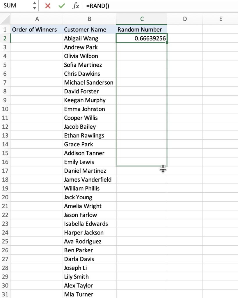
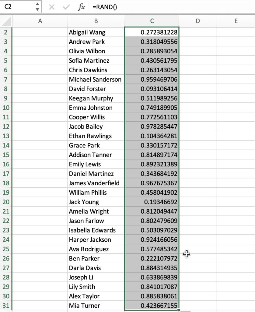
Press ENTER. Drag the formula down to the rest of the rows.
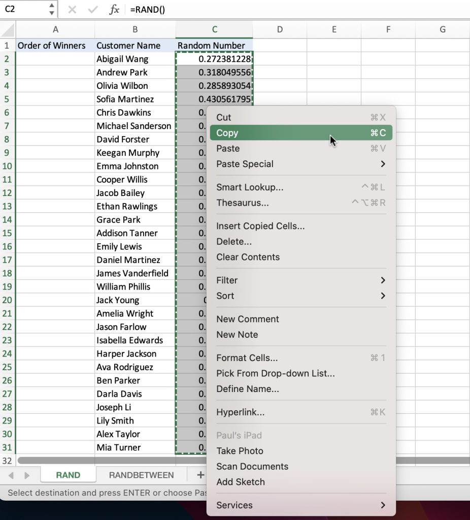
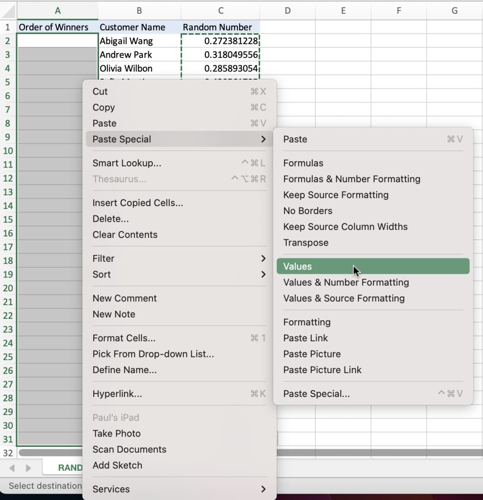
Select the cells with the random numbers and Right-click to Copy.
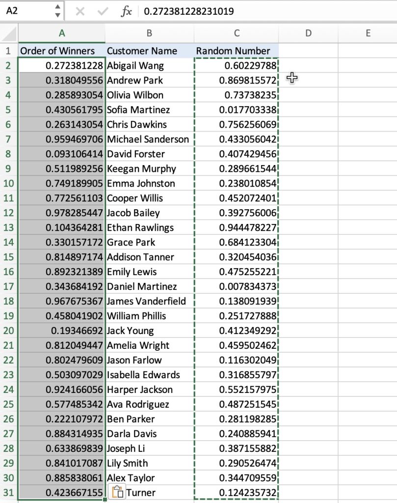
Select cells A2 to A31 and Right-click. Go to Paste Special, then Values.
Note: This step is important because RAND and RANDBETWEEN are volatile formulas and would recalculate every time there is any change in the worksheet.
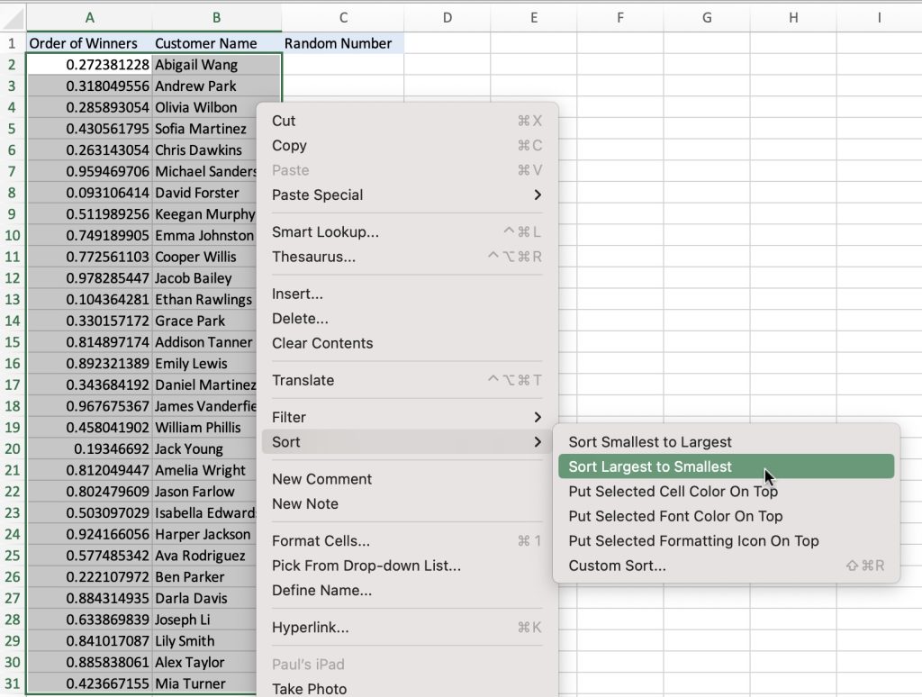
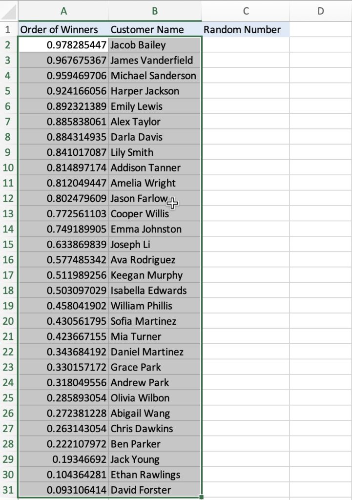
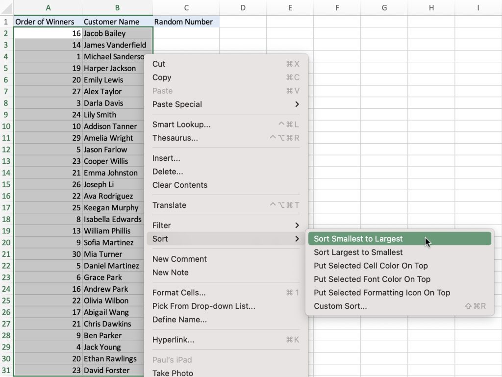
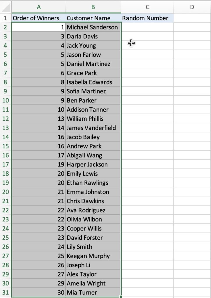
Delete C2 to C31 since RAND will keep generating random numbers. Select A2 to B31 and Right-click. Go to Sort and you can choose between Sort Largest to Smallest or Sort Smallest to Largest.
Select the desired number of customers from the sorted list based on the random numbers assigned to them. For example, if you want to select 10 customers, choose the top 10 customers from the sorted list.
Note: Given the small range (1 to 30) that we are working with, it is possible that duplicate numbers may be generated. However, we can rely on Excel to handle the sorting process and resolve any duplicate values appropriately.
RANDBETWEEN Function: Generating Random Whole Numbers in a Custom Range
What if we want to know how to generate random whole numbers within a chosen range in Excel?
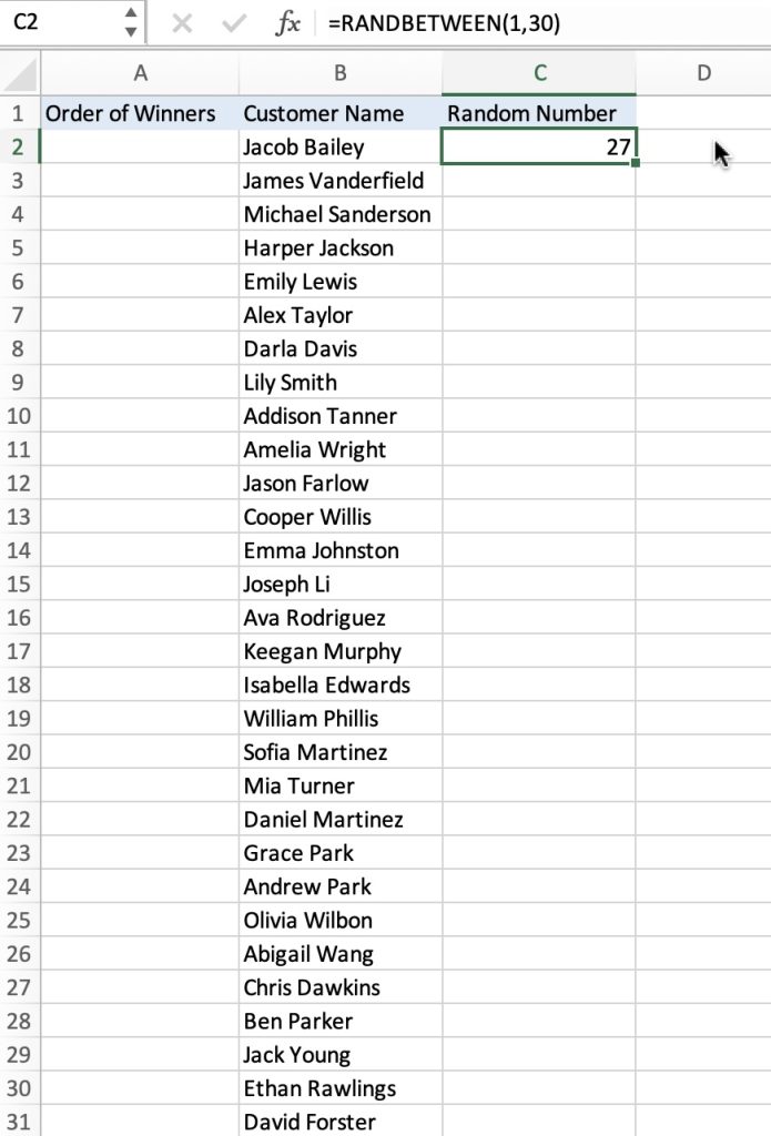
Open an Excel worksheet and create a column labeled Order of Winners in column A, Customer Names in column B, and Random Number in column C. In cell C2, enter the formula =RANDBETWEEN(1,30). This formula generates a random number between 1 and 30.
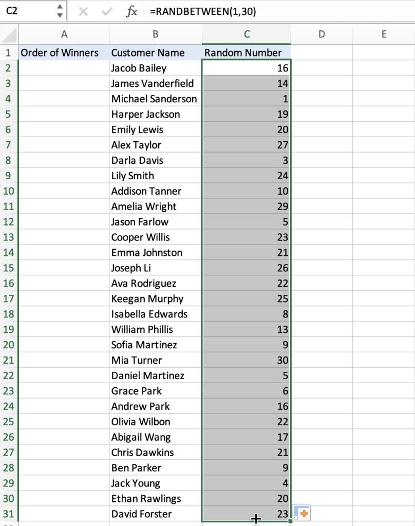
Drag down the formula in cell C2 and paste it into cells C3 to C31 to generate random whole numbers for each customer.
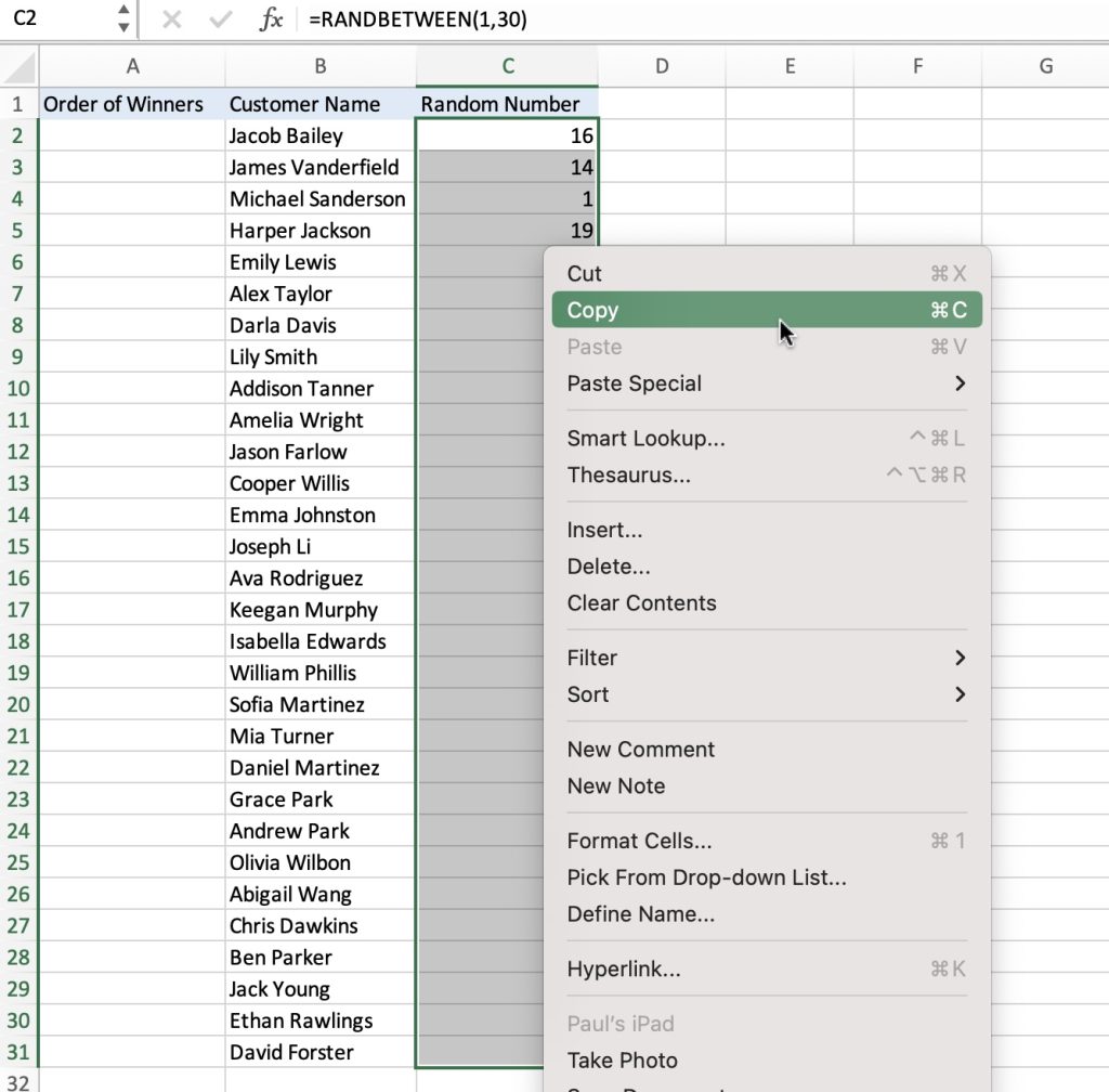
Select C2 to C31 and Right-click. Select Copy.
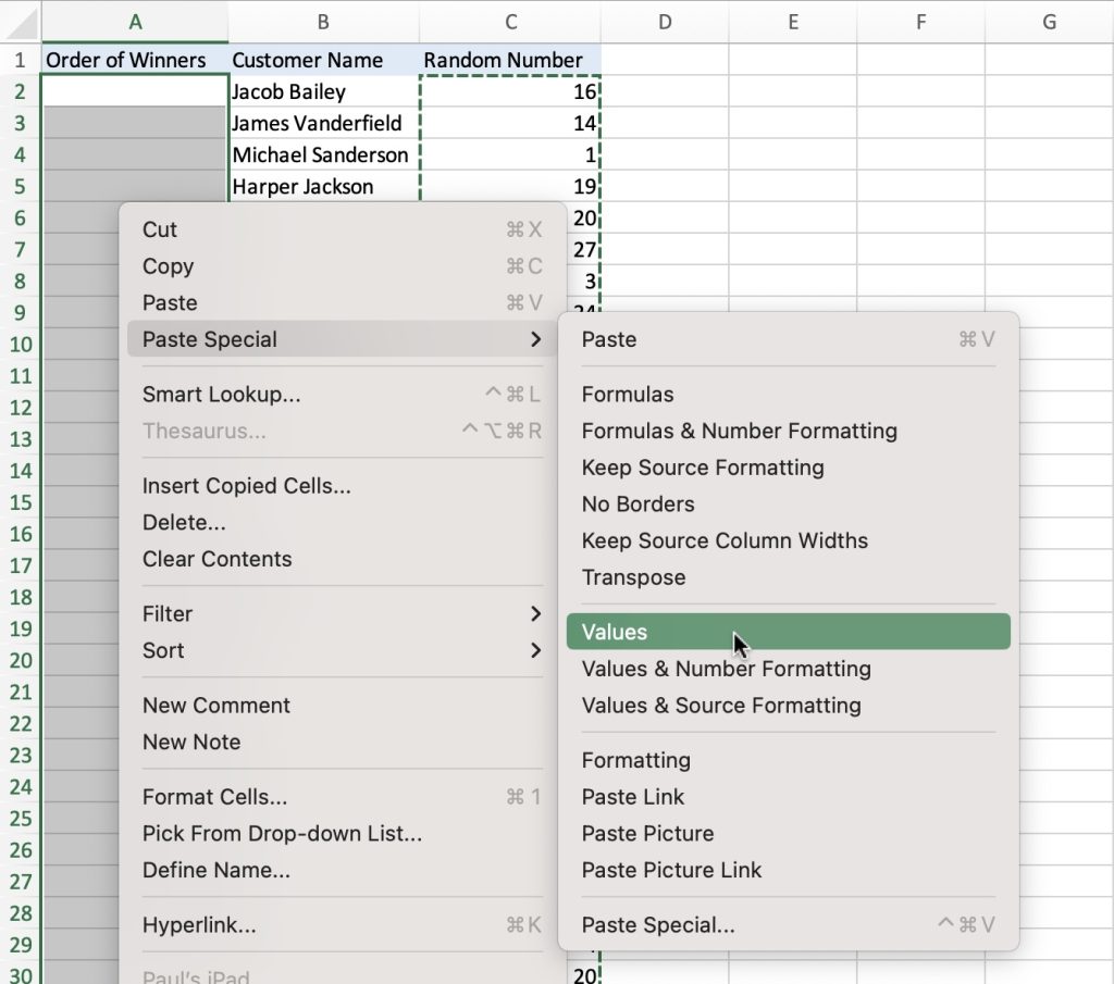
Select cells A2 to A31 and Right-click. Go to Paste Special, then Values.
Delete C2 to C31 since RANDBETWEEN will keep generating random numbers.
Select A2 to B31 and Right-click. Go to Sort and you can choose between Sort Largest to Smallest or Sort Smallest to Largest.
Select the desired number of customers from the sorted list based on the random numbers assigned to them. For example, if you want to select 10 customers, choose the top 10 customers from the sorted list.
There you have it! Excel’s RAND and RANDBETWEEN functions are indispensable tools for small businesses aiming to randomly select customers for special promotions. By understanding how to leverage these functions effectively, you can implement a fair and unbiased customer selection process, boosting engagement and maximizing the success of your promotions. With these methods, you can be assured that you’re promotion will be fair and square. Now, go ahead and apply this to your tasks!
If you want to generate a list of random numbers in an array, click here.
John Michaloudis is a former accountant and finance analyst at General Electric, a Microsoft MVP since 2020, an Amazon #1 bestselling author of 4 Microsoft Excel books and teacher of Microsoft Excel & Office over at his flagship MyExcelOnline Academy Online Course.

