Free Practice Workbook
Conditional formatting is a great tool available in Excel that is used to highlight important information in a large set of data. The various rules include highlighting top values, highlighting duplicate values, and adding color bars or color cells. But sometimes the built-in rules are not enough; this is where formulas come in.
In this article, you will learn how to use conditional formatting with formulas in Excel.
Key Takeaways:
- Conditional Formatting highlights important data automatically.
- Formulas help you create custom formatting rules.
- You can highlight entire rows based on one cell.
- Functions like TODAY and COUNTIF can be used in formulas.
- Conditional Formatting updates when your data changes.
Table of Contents
Introduction to Conditional Formatting
Define Conditional Formatting
Conditional Formatting is a feature that changes the format of a cell based on a specific condition. Instead of manually changing the format of the data, Excel will highlight important values for you. For example, you can highlight sales above $10,000, mark overdue dates in red, identify duplicate entries, or highlight an entire row when a particular condition is met.
When the values in the worksheet change, Excel automatically checks the condition again and updates the formatting.
Conditional Formatting can change several formatting properties, including:
- Cell background color
- Font color
- Font style
- Cell borders
- Number formats
Conditional Formatting Rules
- Highlight Cells Rules: These rules highlight cells based on conditions such as Greater Than, Less Than, Between, Equal To, Text that Contains, A Date Occurring, and Duplicate Values.
- Top/Bottom Rules: These rules help identify values such as the Top 10 Items, Top 10%, Bottom 10 Items, Bottom 10%, Above Average, and Below Average.
- Data Bars: Data Bars display horizontal bars inside cells. Larger values have longer bars, making it easy to visually compare numbers.
- Color Scales: Color Scales use different colors to represent high, medium, and low values.
- Icon Sets: Icon Sets add symbols such as arrows, circles, flags, or ratings based on the value of each cell.
Apply Conditional Formatting with Formula
Step-by-Step Guide
To create Conditional Formatting using a formula, follow the steps below:
- Go to the Home tab

- Select Conditional Formatting > New Rule
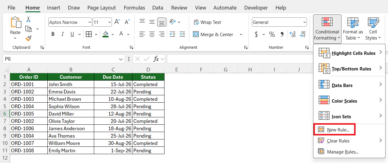
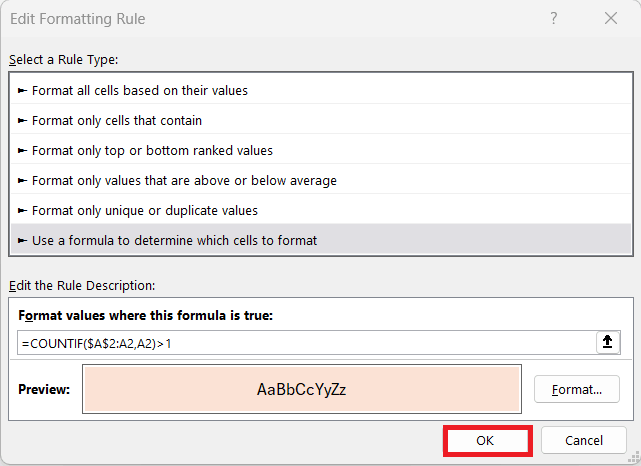
- In the dialog box, select: Use a formula to determine which cells to format
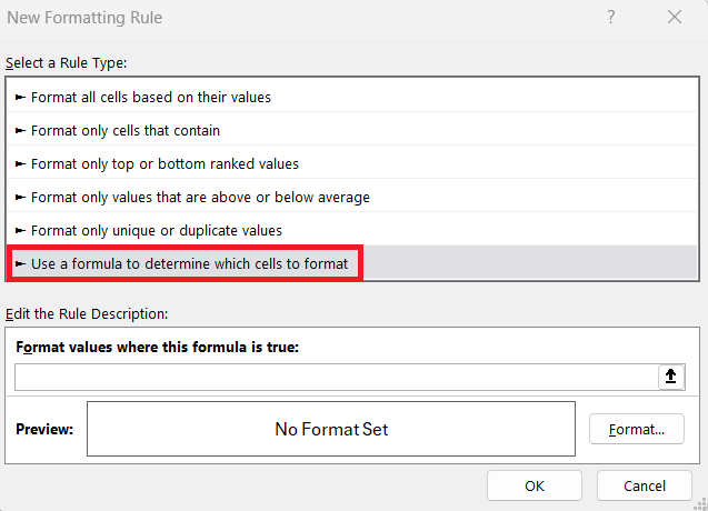
- Enter the formula in the formula box.
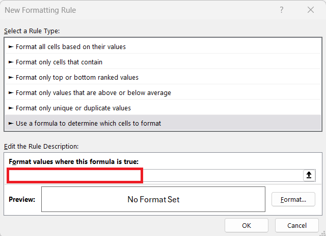
- Click on the Format button
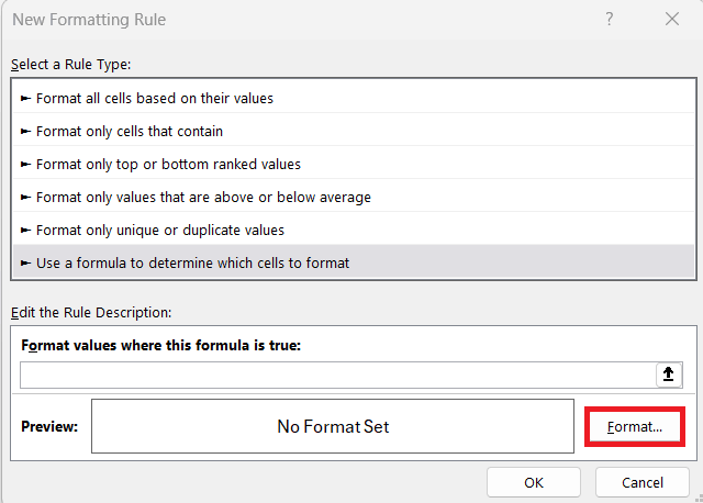
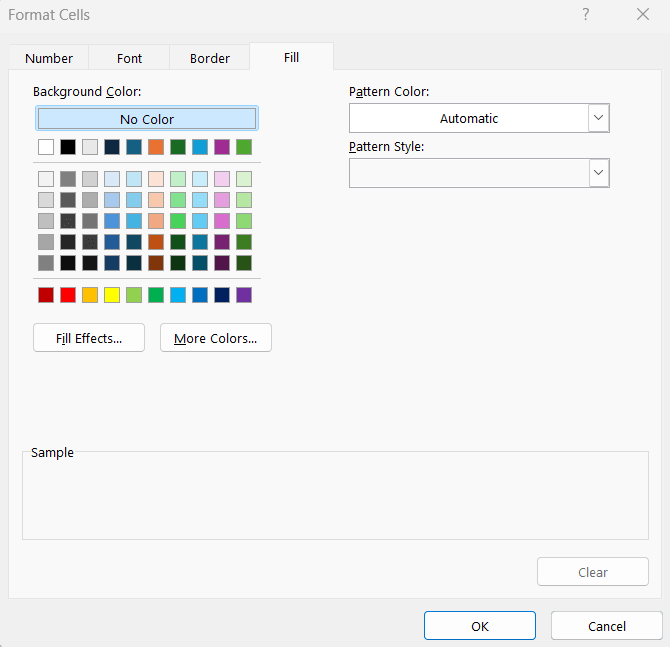
- Choose an appropriate formatting
- Click OK
Example 1: Highlight an Entire Row Based on One Column
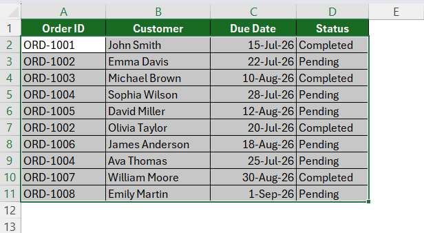
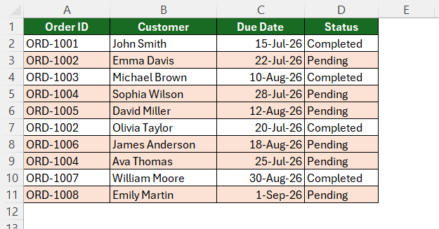
In this example, you have to highlight an entire row if the status is Pending.
- Select the entire data range
- Go to Home > Conditional Formatting > New Rule
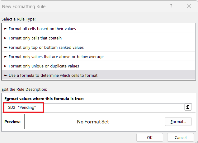
- Select Use a formula to determine which cells to format
- Enter the formula: =$D2=”Pending”
- Click on Format > Select the required fill color > Click OK
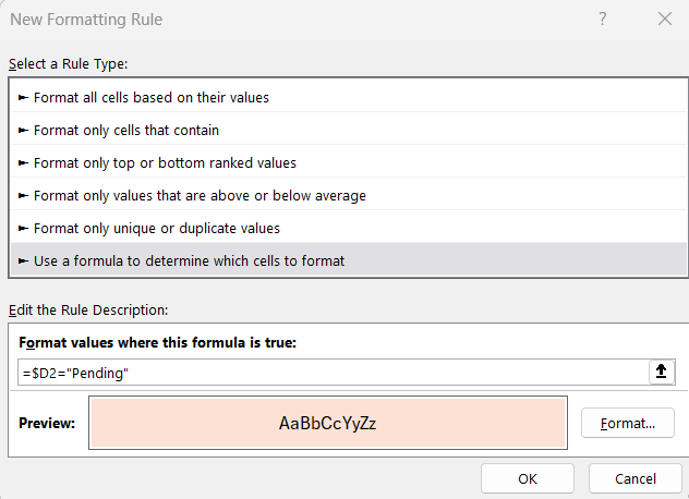
The entire row for an order with status pending will be highlighted.
Example 2: Highlight Overdue Dates
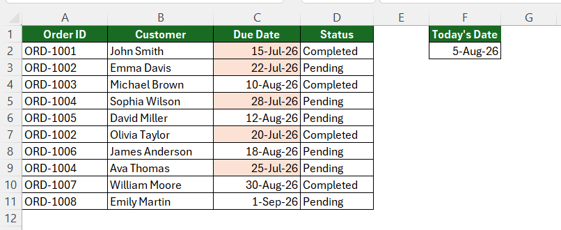
In this example, you have to highlight dates that have already passed.
- Select the Due Data range
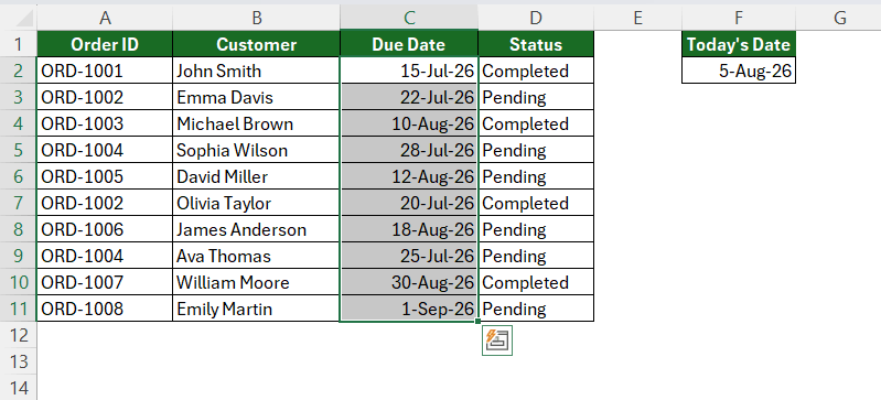
- Go to Home > Conditional Formatting > New Rule
- Select Use a formula to determine which cells to format
- Enter the formula: =B2<TODAY()
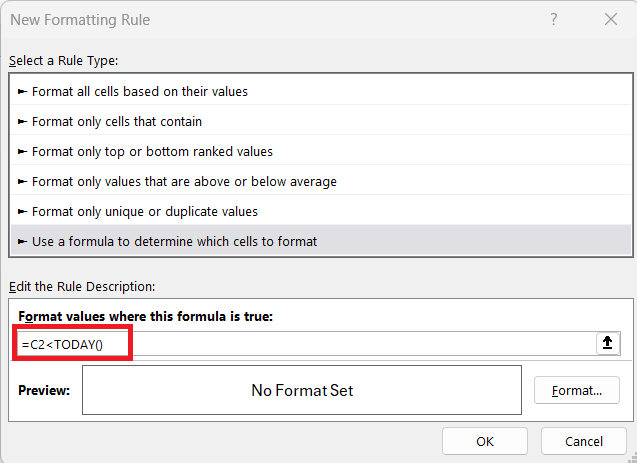
- Click on Format > Select the required fill color > Click OK
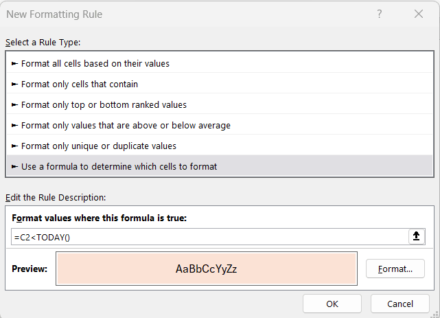
Excel highlights any date that is earlier than today’s date.
Example 3: Highlight Repeat Entries Only
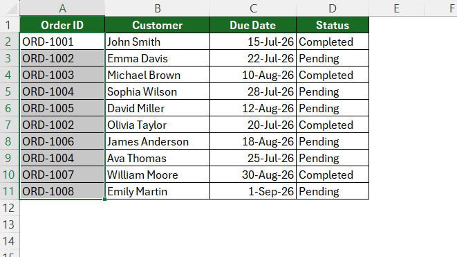
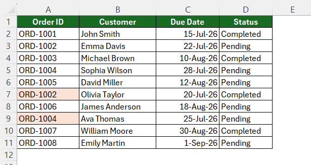
Excel already provides a built-in rule for highlighting duplicate values. However, formulas provide more control. It will highlight repeated entries and leave the first occurrence unchanged.
- Select the Order ID range
- Go to Home > Conditional Formatting > New Rule
- Select Use a formula to determine which cells to format
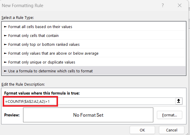
- Enter the formula: =COUNTIF($A$2:A2,A2)>1
- Click on Format > Select the required fill color > Click OK
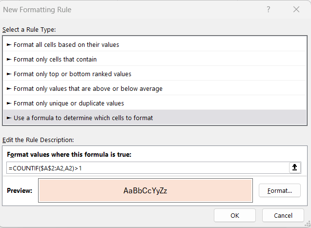
Excel highlights the second or more occurrences.
Manage Conditional Formatting Rules
As you add more Conditional Formatting rules, it is important to manage them properly.
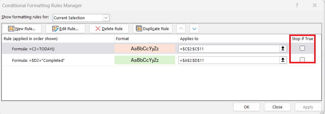
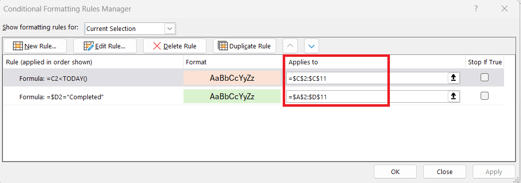
Go to Home > Conditional Formatting > Manage Rules
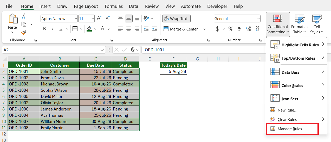
Here, you can create a new rule, edit an existing rule, or delete a rule.
- Rule order – Excel checks rules from the top of the list downward. You can use the arrow keys to change the order of the rule.
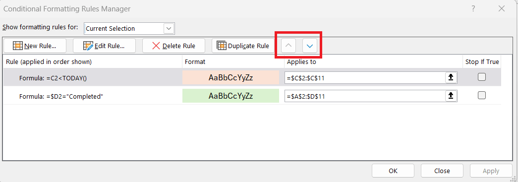
- Stop if True – Tick this box, and Excel stops checking any lower rules for a cell once this rule matches.
- Applies to – This column shows the range covered by each rule.
FAQs
1. What is Conditional Formatting in Excel?
Conditional Formatting changes the format of cells when specific conditions are met.
2. Can I use a formula in Conditional Formatting?
Yes. You can use formulas to create custom formatting rules.
3. Can Conditional Formatting highlight an entire row?
Yes. A formula can highlight an entire row based on a value in one column.
4. How to edit a Conditional Formatting rule?
Go to Home > Conditional Formatting > Manage Rules and select the rule you want to edit.
5. Does Conditional Formatting update automatically?
Yes. Excel updates the formatting automatically when the cell values change.

John Michaloudis is a former accountant and finance analyst at General Electric, a Microsoft MVP since 2020, an Amazon #1 bestselling author of 4 Microsoft Excel books and teacher of Microsoft Excel & Office over at his flagship MyExcelOnline Academy Online Course.

 30 Days - Full Access