Dynamic Data List using Excel Tables

Microsoft Excel is widely used for data management, reporting, and analysis across industries. One of its most powerful, yet often underutilized, features is the ability to create dynamic data lists using Excel Tables. Dynamic lists not only make data entry faster but also reduce errors, improve efficiency, and ensure that your spreadsheet adapts automatically as new data is added. In this article, we will explore what dynamic data lists are, why they are useful, and provide a detailed, step-by-step guide to creating a Dynamic Data List using Excel Tables.

Key Takeaways:

• Dynamic data lists automatically update as new data is added to the Excel Table.
• They reduce data entry errors by restricting input to predefined values.
• Named ranges linked to tables make formulas and references easier to manage.
• Drop-down lists created from tables improve efficiency and user experience.
• Advanced tips like sorting, unique lists, and combining columns enhance list functionality.

Download excel workbookDynamic-Data-Validation.xlsx

 

Understanding Dynamic Data List

What is a Dynamic Data List?

A dynamic data list is a list in Excel that automatically updates when new items are added to the source data. Unlike static lists, which are fixed in size, dynamic lists grow or shrink as your data changes. This means you don’t have to manually update your drop-down menus, named ranges, or formulas every time you add a new entry.

For example, imagine you have a list of products in your Excel file. If you want users to select a product from a drop-down list, a static list would require manual updates every time a new product is added. With a dynamic data list, Excel automatically includes any new products added to the table, ensuring your drop-down menu is always up-to-date.

Why Use Dynamic Data Lists?

Dynamic data lists are valuable in several scenarios:

• Prevent Data Entry Errors: Drop-down lists restrict user input to predefined values, reducing spelling mistakes, duplicates, and inconsistent entries.
• Improve Efficiency: Users can quickly select values from a list rather than typing manually. This is especially useful in forms, surveys, or large datasets.
• Automate Updates: When your list grows over time, a dynamic list automatically adjusts. You no longer need to redefine ranges or manually update data validation rules.
• Professional Reporting: Dynamic lists improve spreadsheet design and make dashboards more interactive. Users can select from valid options that are always current.
• Simplify Formulas and References: Named ranges linked to Excel Tables simplify formula references, making spreadsheets easier to manage.

 

Step-by-Step Guide to Creating a Dynamic Data List Using Excel Tables

Here is how to create a dynamic data validation list using Excel Tables:

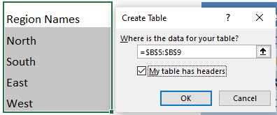
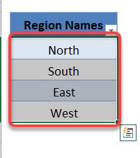
STEP 1:  Convert your list in to an Excel Table (Ctrl+T)

STEP 2: Select your Table column by hovering over the Excel Table and left clicking when the arrow pointer shows

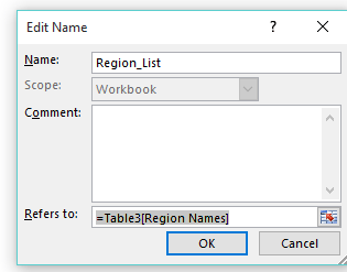
STEP 3: In the ribbon menu, go to Formulas > Define Name > enter a custom name with no spaces (we will put this name in step 5) and press OK

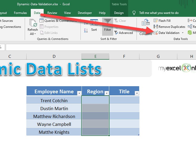
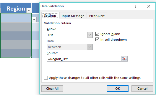
STEP 4: Click on the other Excel Table column that you want to enter the dynamic list into and go to the ribbon and choose Data > Data Validation > List

STEP 5: In the Source box, enter the name you created in Step 3 and press OK, or click in the Source box, press F3, and select the named range from there (thanks to Michael from www.excelpogodzinach.pl for introducing this tip to us!)

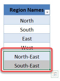
STEP 6: If you want to add extra data into your Excel Table list, hover with your mouse in the bottom right hand corner and when you see a double arrow, drag down.

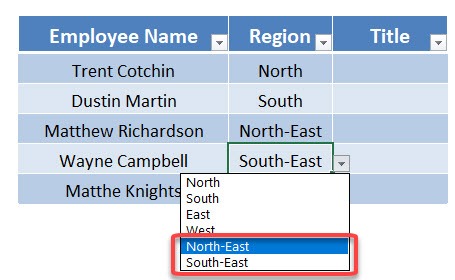
STEP 7: Enter a new entry, and this will automatically be updated in your drop-down list.

 

Advanced Tips for Dynamic Data Lists

1. Sort the List Automatically

Keep your list organized by sorting it alphabetically or numerically. Use the filter arrow in the table header or the SORT() function in modern Excel. The drop-down updates automatically to reflect the new order.

2. Use Unique Lists

Sometimes, your source table may contain duplicates. To create a drop-down with only unique entries, use Excel’s Remove Duplicates feature or leverage the UNIQUE() function in modern versions of Excel.

=UNIQUE(ProductsTable[ProductName])

This ensures only distinct values appear in your list.

3. Combine Multiple Columns

For drop-downs showing combined data (e.g., “Product – Category”), create a helper column using & or TEXTJOIN():

=TEXTJOIN(” – “, TRUE, A2:B2)

Convert this column into a table for a dynamic list.

4. Handle Errors Gracefully

Use Input Messages to guide users and Error Alerts to prevent invalid entries. Example: “Please select a product from the drop-down list.”

 

FAQs

Q1: What is a dynamic data list in Excel?

A dynamic data list is a list that automatically updates whenever new items are added to the source table. Unlike static lists, it grows or shrinks as your data changes. This ensures drop-down menus always reflect current data. It eliminates the need to manually update named ranges or formulas. Dynamic lists are ideal for forms, surveys, and dashboards.

Q2: How do I create a dynamic drop-down list using an Excel Table?

First, convert your source list into an Excel Table using Ctrl + T. Then, define a named range for the table column. Next, select the target column, go to Data > Data Validation > List, and enter the named range as the source. Finally, any new entries added to the table automatically appear in the drop-down. This process ensures your list is always up-to-date.

Q3: Can I prevent duplicates in my dynamic list?

Yes, you can remove duplicates from the table using Data > Remove Duplicates. In modern Excel versions, you can also use the UNIQUE() function to create a dynamic array of distinct values. This ensures your drop-down only contains unique entries. Maintaining unique values reduces errors and improves clarity. It’s especially useful for employee names, products, or categories.

Q4: How can I combine multiple columns in a drop-down list?

You can create a helper column that concatenates values using & or the TEXTJOIN() function. For example, =TEXTJOIN(” – “, TRUE, A2:B2) combines two columns with a delimiter. Convert this helper column into a table to maintain dynamic behavior. Your drop-down will now show combined entries like “Product – Category.” This is useful for dashboards or reports with multiple attributes.

Q5: How do I handle errors when users enter invalid data?

Use Data Validation Input Messages to guide users on valid selections. Enable Error Alerts to prevent invalid entries and display a custom warning, such as “Please select a product from the list.” This reduces mistakes and keeps data consistent. Input messages improve user experience by providing guidance before entry. Combined with dynamic lists, this ensures accurate and reliable data collection.