How to Utilize LEFT Function for Data in Excel – Step by Step Guide

In the realm of data analysis, the Excel LEFT function emerges as a simple yet powerful tool. By extracting specific characters from the left side of a text string, it can streamline tasks and reveal insights buried within large datasets. This function can save you time and enhance precision in your data manipulation efforts.

Key Takeaways:

• The LEFT function extracts characters from the left side of a text string.
• It’s highly useful for simplifying and standardizing text data.
• The function works well with other Excel tools like FIND and LEN.
• Proper syntax and understanding of the num_chars argument are crucial.
• LEFT can face challenges with dates, but these can be resolved with the TEXT function.

 

Mastering Data with Excel’s LEFT Function

Unveiling the Power of LEFT in Data Analysis

In my experience diving deep into data analysis, I’ve discovered that Excel’s LEFT function is a hidden gem often overlooked. Yet, it wields significant power to streamline workflows, particularly when we’re wrestling with large datasets.

By deftly extracting specific characters from a mass of text data, LEFT simplifies what would otherwise be a daunting task, enabling quick interpretations, comparisons, and transformations of data.

Navigating the Basics: What is the LEFT Function?

The LEFT function is an essential tool in Excel’s robust arsenal for text manipulation. It allows us to pull out a designated number of characters from the leftmost part of a text string. This functionality is critical when we need to isolate specific information from a cell that contains a combination of data.

Imagine you’re faced with a cluttered spreadsheet; the LEFT function can be your ally in extracting readable, usable information from that chaos.

 

The Backbone of LEFT: Understanding Syntax and Arguments

Breaking Down the Syntax: A Step-by-Step Explanation

Delving into the LEFT function’s syntax reveals its straightforward logic. The function follows a simple formula: =LEFT(text, [num_chars]).

• text represents the string from which characters will be extracted, and
• [num_chars] denotes the number of characters to retrieve from the left side of the string.

This optional argument defaults to 1 if omitted, grabbing just the first character. The elegance of LEFT lies in its minimalism; with just two parameters, we can perform powerful text extractions tailored to our analytical needs.

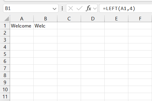
For example, if cell A1 contains the text “Welcome,” the formula =LEFT(A1,4) will return “Welc”.

The Significance of Num_chars and How to Use It

The num_chars argument in the LEFT function is what allows us to tailor the output to our specific needs. Its significance cannot be overstated — it defines the exact breadth of text to be extracted, ensuring precision in data manipulation. To use it effectively, we provide a positive integer that dictates the number of characters to extract from the left.

If we need to extract a dynamic number of characters based on another cell’s value, we can reference a cell for num_chars. This makes the LEFT function adaptable to varying contexts within our spreadsheet. Always ensure num_chars is positive; a negative will throw an error, a pitfall easily avoided with foresight in your formula crafting.

 

Practical Applications: Making the Most of LEFT

Simplifying Text Data: Examples and Use Cases

The LEFT function in Excel is a valuable tool for extracting a specific number of characters from the beginning of a text string. This feature is especially useful in data cleaning, formatting, and preparation tasks, where simplifying or standardizing text data is crucial. Below are some detailed examples and creative ways to leverage the LEFT function in your Excel projects.

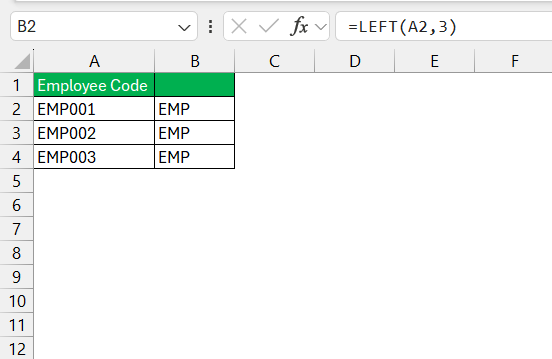
1. Extracting Prefixes: Many organizations use standardized prefixes in their data, such as employee IDs, product codes, or project identifiers. For instance, consider employee IDs formatted as “EMP001,” “EMP002,” and so on. If you need to extract just the “EMP” portion from each ID for categorization or reporting purposes, you can use the formula =LEFT(A2,3).

This formula instructs Excel to take the first three characters from the text in cell A2, effectively isolating the “EMP” prefix. This can be particularly useful when sorting or filtering data based on these prefixes.

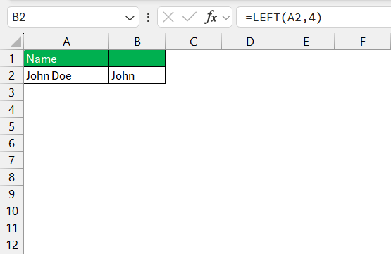
2. Isolating Names or Initials: When dealing with full names, such as “John Doe,” you might only need to extract the first name for a personalized greeting or to create a list of first names. Using the formula =LEFT(A3,4) will return “John,” assuming A3 contains “John Doe.”

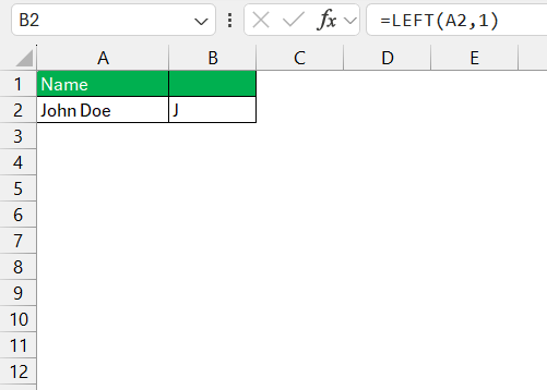
This approach is also helpful when you need to generate initials. For example, extracting the first initial from “John Doe” can be done with =LEFT(A3,1), which returns “J.”

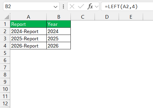
3. Extracting Dates from Text: In some datasets, dates might be embedded within text strings, like “2024-Report”. If you need to extract the year, you can use =LEFT(A1,4) to get “2024”. This can be particularly useful for sorting or filtering data by year.

Creative Combinations: Integrating LEFT with Other Functions

The LEFT function’s versatility increases dramatically when combined with other Excel functions. Here are some advanced uses:

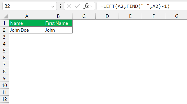
1. LEFT with FIND: Sometimes, you need to extract text up to a specific character, such as a hyphen, space, or comma. For example, if cell A2 contains “John Doe,” and you want to extract just “John,” you can combine LEFT with the FIND function: =LEFT(A2,FIND(" ",A2)-1).

The FIND function locates the position of the hyphen, and LEFT extracts everything before it. This combination is powerful for text that follows a predictable pattern, making it easier to parse and analyze.

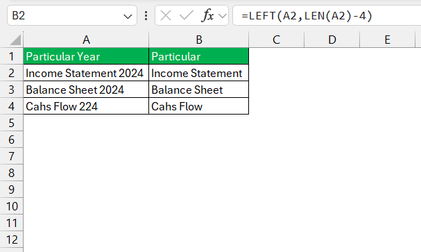
2. LEFT with LEN: When dealing with varying text lengths, combining LEFT with LEN (which returns the length of a text string) can be useful. For instance, if you have a string where you want to remove the last few characters, you can subtract a fixed number from the total length: =LEFT(A2,LEN(A2)-4) would remove the last four characters from the text in A2.

This combination is particularly helpful when standardizing text lengths across different entries in your dataset.

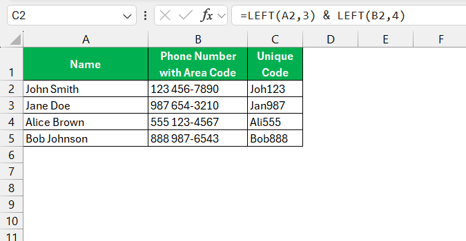
3. LEFT with CONCATENATE: You can also use LEFT in conjunction with CONCATENATE (or the & operator) to dynamically build new strings. For example, if you need to create a unique identifier by combining the first three letters of a name with the first three digits of a phone number, you can use =LEFT(A2,3) & LEFT(B2,4) where A2 contains the name and B2 is the phone number.

 

Troubleshooting Common LEFT Function Issues

Overcoming Error Messages and Unexpected Results

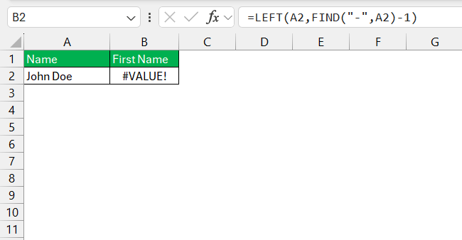
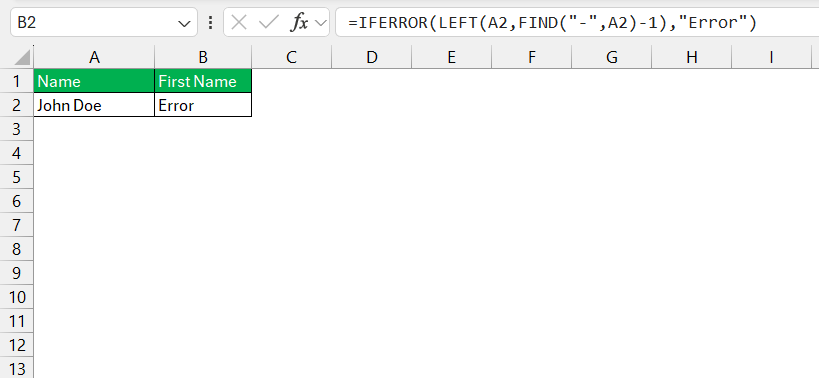
When combining LEFT with FIND, if the character you’re searching for (e.g., a hyphen) isn’t present in the text, FIND will return an error.

To prevent this from disrupting your workflow, wrap your formula in IFERROR(), like this: =IFERROR(LEFT(A2,FIND("-",A2)-1),"Error"). This formula ensures that if the hyphen isn’t found, the formula will return an empty string instead of an error.

Best Practices

• Always Check Your Lengths: Be mindful of the num_chars argument in your LEFT function. If you request more characters than the text contains, Excel will still return the full text without errors, but you may end up with unnecessary spaces or incomplete extractions. Always tailor the number of characters to match your data’s structure.
• Data Consistency: Before using the LEFT function, ensure your data is consistent and clean. Extra spaces, unexpected characters, or inconsistent text lengths can lead to errors or misinterpretations. Use Excel’s TRIM() and CLEAN() functions to remove unwanted characters and spaces from your data before applying LEFT.

 

FAQs: Enhancing Your Understanding of LEFT

How do you use the left function in Excel?

To use the LEFT function in Excel, you first select the cell where you want the result to appear, then type in `=LEFT(text, num_chars)` where `text` is the reference to the cell with the string you want to extract from, and `num_chars` is the number of characters you want to extract from the left side of the string. Alternatively, you can use the Excel dialog box by clicking on the “Text” tab under the “Formulas” tab and then selecting “LEFT” to input your arguments and attain the formula result.

How do I remove 3 characters from left in Excel?

To remove 3 characters from the left side of a text in Excel, you can use the `LEFT` function combined with `LEN`. For example, if you want to remove 3 characters from the text in cell A1, you would use the formula `=RIGHT(A1, LEN(A1)-3)`. This formula uses the `RIGHT` function to return the text from A1 after omitting the first 3 characters.

How do you extract the first 4 characters in Excel?

To extract the first 4 characters from a string in Excel, you can use the LEFT function by inputting `=LEFT(A1, 4)` into a cell formula, where `A1` is the cell reference containing the string. This function will return the first 4 characters from the specified string in cell A1. If you want to extract from a different cell, replace `A1` with the appropriate cell reference.

Why Isn’t LEFT Working with Dates and How Can I Fix It?

LEFT doesn’t play well with dates because dates in Excel are stored as serial numbers; thus, applying LEFT directly to a date often results in extracting the starting digits of its underlying number—not the actual date components we see. But fear not, to fix it, you can nest the TEXT function within LEFT, formatting the date as a text string first. For example, =LEFT(TEXT(A1,"dd/mm/yyyy"), 2) would fetch the day from a date in cell A1. Another approach is to use dedicated Excel date functions such as DAY, MONTH, or YEAR to extract the respective parts.