The subtotal function in Microsoft Excel is a versatile tool designed to simplify data analysis by performing a variety of calculations, such as sums, averages, and counts, on a specified range of cells. Unlike the standard SUM function, Subtotal can dynamically include or exclude hidden and filtered rows, making it ideal for working with dynamic datasets. This powerful feature allows users to efficiently manage and analyze large sets of data with precision and ease.
See how this is done by following this Excel workbook:
Download workbookSubtotal-Visible-or-Filtered-Values.xlsx
Unveiling the Magic of Excel’s Subtotal Function
What Is the Subtotal Function?
Imagine having a wizard at your fingertips to effortlessly crunch numbers, weaving in and out of data with precision and speed. That’s what the Subtotal function in Excel feels like—a spell that conjures up a variety of calculations on your dataset with simplicity and agility.
Imagine you have a range of cells, each brimming with numbers. Instead of applying multiple formulas to sum up or average these figures, the Subtotal function is your go-to tool. It deftly calculates everything from sums to averages, counts to max values, all while allowing you to either factor in or ignore rows that you’ve decided to hide manually.

Decoding the Syntax and Parameters
In the grand library of Excel functions, the ancient scrolls reveal the following incantation for the SUBTOTAL function:
Here’s the key to unlocking its power:
method: This mystical parameter determines the type of calculation the SUBTOTAL function will perform. Excel recognizes a variety of numerical codes—1 for average, 2 for count, 3 for counta, and so forth up to 11. If you require subtotal to consider only visible data, cast the incantation with codes 101 to 111.range1, [range2, ... range_n]: These are the cells over which the SUBTOTAL function will wave its wand. You can specify one or more ranges, and it doesn’t shy away from multiple areas. Just remember, these ranges must be separated by commas in this arcane formula.
When woven correctly, this formula allows you to consolidate your data like a seasoned sage, transforming entire columns and rows with a simple spoken word—or rather, a simple input in Excel’s function bar.
Example

The formula =SUBTOTAL(1,B2:B6) in Excel is used to calculate a subtotal for a specified range of cells, in this case, the range B2:B6. The SUBTOTAL function is quite versatile and can perform different types of calculations based on the function number provided as the first argument.
Here’s a breakdown of the formula components:
- SUBTOTAL: The function that performs a variety of aggregate calculations on a specified range.
- 1: The function number that specifies which type of calculation to perform. The number 1 corresponds to the AVERAGE function.
- B2:B6: The range of cells on which the subtotal calculation will be performed.
So, =SUBTOTAL(1,B2:B6) calculates the average of the values in the range B2:B6.
Harnessing the Power of Subtotal in Excel
Step-by-Step Guide to Inserting Subtotals
Injecting subtotals into your Excel sheets is an expedition that’ll take you just a few clicks. Here’s a compass to guide you through:
STEP 1: Select Your Data: Before summoning subtotals, ensure your data is sorted and selected based on the column you want to subtotal. Remember, no blank rows should lurk between your data; they could disrupt the spell.

STEP 2: Begin the Magic: Navigate to the ‘Data’ tab and find the ‘Subtotal’ button tucked in the ‘Outline’ group. It’s the gateway to your data transformation.

STEP 3: Subtotal Dialog Box: This is where the enchantment happens. The dialog box will ask you to select the magic words (‘At each change:’ in as ‘Region’), the sorcery you wish to perform (choose ‘Sum’), and the potion concoction (‘Add subtotal to:’ as ‘Sales’).

STEP 4: Refine the Spell: Ensure that ‘Replace current subtotals’ is checked if you want to overwrite any previously cast subtotal spells. You wouldn’t want the old and new magics to clash. Then click, ‘OK’.

RESULT: Finalize Your Incantation: With a swift click on ‘OK’, watch as the rows bend to your will, arranging themselves with neat subtotals as demanded.

If your dataset has multiple portals needing the touch of subtotal magic, repeat the steps for each. Think of it as creating layers of spells, one atop another, for a multi-dimensional view of your numbers.
Advanced Techniques with Nested Subtotals
As you delve deeper into the sorcery of Excel, nested subtotals emerge as your wand for crafting a masterful financial analysis spellbook. Here’s how to summon these advanced enchantments:
- Layer Your Sorts: Start by ordering your cauldron’s contents—sort your data by the most outer group first (say, ‘Region’), then by the subsequent inner groups (like ‘Item’). Each layer prepares the potion for more complex flavors.
- Insert the First Subtotal Layer: Select any cell in your dataset, then activate the Subtotal command. Choose your first group (like ‘Region’) for the ‘At each change in’ field, pick the potion—’Sum’ to amass wealth, ‘Average’ to find the golden mean, and so on. Choose your treasures, the columns filled with riches, to apply the function.
- The Art of Collapsing: Use the grouping outlines on the left to fold and unfold the layers of your analysis. Revel in how it reveals or conceals information, offering insights at different levels, from the grand overview to the detailed underside.
The dexterity lies in the balance; carefully layering subtotals can yield a magical mirror reflecting every facet of your financial realm, making it a crystal ball to foresee and navigate through the numerals of fate.
Tricky Terrain: Troubleshooting Common Errors
Identify and Fix Excel Subtotal Glitches
Stumbling into the occasional spellbinding issue with SUBTOTAL in Excel is as inevitable as a cauldron bubbling over — it happens to the best of wizards. Here’s how to identify and rectify some common glitches:
- #NAME?: If the cells whisper this incantation error, it means you’ve likely misspelled “SUBTOTAL” — a simple misstep on the spelling spell. To set it right, perform a quick spell-check and correct the function name.

- #VALUE!: This one’s tricky as it suggests your function number isn’t in the range 1-11 or 101-111, or you’ve included a three-dimensional charm where a flat spell was expected. To banish this error, double-check your function_num argument and pare down your references to the second dimension only.

- #DIV/0!: This happens when a particular function, such as calculating an average or standard deviation, attempts to divide by zero within a range of cells that don’t contain any numeric values.

By keeping a vigilant eye out for these anomalies and a steady hand ready to correct them, you ensure that your Subtotal function weaves a flawless tapestry of numbers and data.
How to Include Hidden Values
The SUBTOTAL function in Excel has many great features, like the ability to:
- Return a SUM, AVERAGE, COUNT, COUNTA, MAX or MIN from your data;
- Find the SUBTOTAL of filtered values;
- Ignore other SUBTOTALS that are included in your range, avoiding any double counting!
- Include hidden values within your data by entering the first argument function_num, as values between 1-11;
- Ignore hidden values within your data by entering the first argument function_num, as values between 101-111;
- Sometimes you are faced with lots of data and just want to show the Totals row and hide all the individual rows that make up the Totals, just for presentation purposes.
Using the SUBTOTAL function you can Sum your list of values and then hide them from the worksheet without affecting the function.
STEP 1: function_num: For the 1st argument, select a number from 1-11, which will include any manually hidden rows in the SUBTOTAL calculation!
STEP 2: ref1: For the 2nd argument, select the range of values that you want to use in your SUBTOTAL calculation.
STEP 3: Highlight the values that you do not want to show on your worksheet and then Right Click and select Hide.
See how this is done by following this simple tutorial:
Download workbookSubtotal-Hidden-Visible-Values.xlsx
***Values for the SUBTOTAL function_num:
| Includes hidden values | Ignores hidden values | Function |
| 1 | 101 | AVERAGE |
| 2 | 102 | COUNT |
| 3 | 103 | COUNTA |
| 4 | 104 | MAX |
| 5 | 105 | MIN |
| 6 | 106 | PRODUCT |
| 7 | 107 | STDEV |
| 8 | 108 | STDEVP |
| 9 | 109 | SUM |
| 10 | 110 | VAR |
| 11 | 111 | VARP |
How to Include Filtered or Visible Values in Your Subtotal
Whenever you have a list of data with a filter (CTRL+SHIFT+L) and want to Sum a column, entering a SUM function works fine but it gives you the wrong result whenever you select a filter within your data.
That is because a SUM function includes the hidden values in the calculation. Not to worry, SUBTOTAL to the rescue!
Using the SUBTOTAL function you can Sum your list of values, then filter your list which returns the Sum of only the visible or filtered values.
STEP 1: function_num: For the 1st argument, select a number from 101-111, which will ignore any hidden values in the SUBTOTAL calculation!

STEP 2: ref1: For the 2nd argument, select the range of values that you want to use in your SUBTOTAL calculation.
FAQ – Your Questions Answered
What is the subtotal in Excel?
In Excel, the subtotal is like your trusty Swiss Army knife for data analysis. It lets you quickly calculate summary statistics like sums, averages, or counts for subsets of your data while allowing the option to include or exclude filtered and hidden rows in the calculations. It’s a formula, using the SUBTOTAL function, that flexes to your needs and keeps your data analysis sharp and concise.
How is subtotal different from sum Excel?
Subtotal in Excel is a seasoned traveler through your data, whereas Sum is more of a homebody. Sum tallies all numbers in a range, without discretion. Subtotal, on the other hand, is selective—it can perform the same sum operation while optionally ignoring rows you’ve hidden or filtered out, making it ideal for dynamic, changing datasets. [Include screenshot showcasing SUM vs. SUBTOTAL with filtered data].
How Do I Only Calculate Visible Cells Using SUBTOTAL?
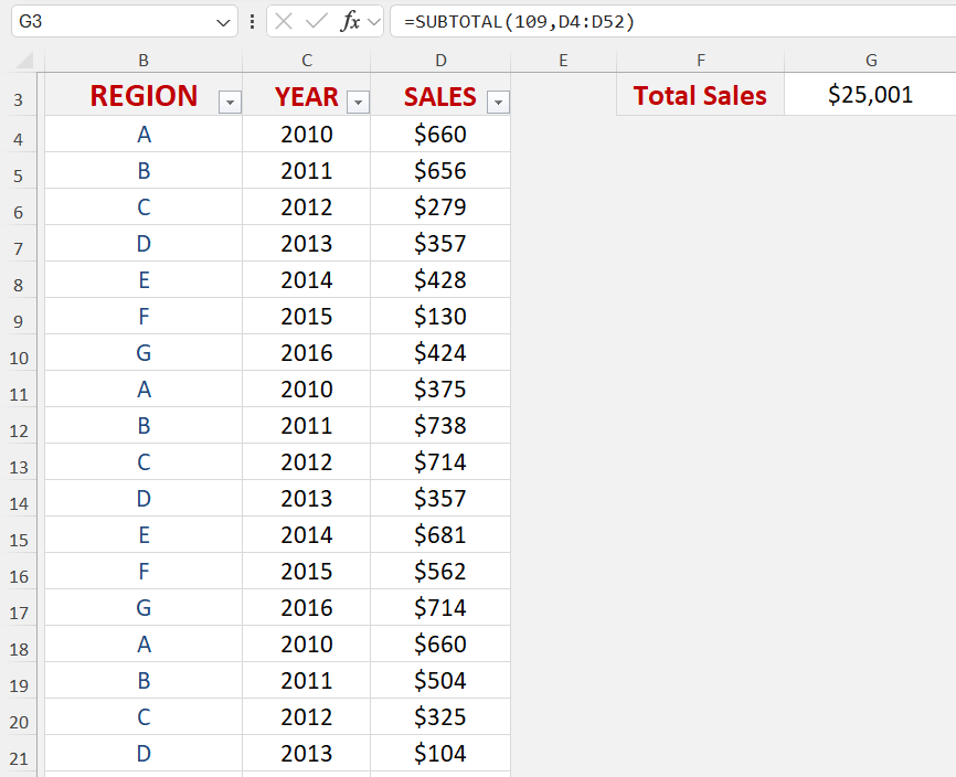
To calculate only visible cells in Excel, embrace the SUBTOTAL function with codes 101-111, like 109 for sum. These codes tell SUBTOTAL to become a seer, turning its gaze only to what is visible, ignoring the hidden rows shrouded by filters or manual concealment with eagle-eyed precision.
Can You Explain the Difference Between SUBTOTAL 9 and 109?
Certainly! Imagine SUBTOTAL function numbers as two different keys to the same door. SUBTOTAL 9 opens up to include both visible and manually hidden rows in its calculation. Meanwhile, SUBTOTAL 109 is a more selective key, ignoring the rows you’ve tucked away out of sight and only accounting for the ones in plain view. Both calculate the sum, but with a slight twist in visibility.
How to subtotal in Excel excluding hidden rows?
To subtotal in Excel while excluding hidden rows, use the crafty SUBTOTAL function with codes 101-111. For sum, it’s 109; for average, 101. These special codes let SUBTOTAL know you wish to leave out those sneaky hidden rows from your totals, focusing only on the rows that bathe in the light of your spreadsheet.

John Michaloudis is a former accountant and finance analyst at General Electric, a Microsoft MVP since 2020, an Amazon #1 bestselling author of 4 Microsoft Excel books and teacher of Microsoft Excel & Office over at his flagship MyExcelOnline Academy Online Course.


