Table of Contents
Filter a Pivot Table by Dates
There are an array of different Date filters in a Pivot Table. You can filter by a particular date range, for example: by this week, next month, next quarter, next year, last year, year to date and the list goes on and on. This is useful if you want to see what invoices are due to be paid this month or what sales transactions were included in a particular quarter.
Below I show you a few quick Pivot Table filter examples.
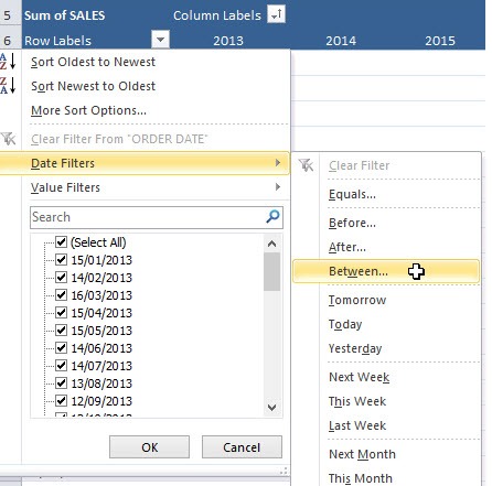
STEP 1: Go to Row Labels and select Date Filters > Between
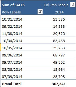
STEP 2: Place a date range. Click OK.
Your pivot table is now filtered by the dates!
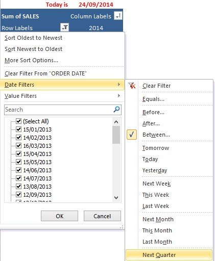
STEP 3: Let us try another one. Go to Row Labels and select Date Filters > Next Quarter
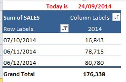
Your pivot table is now filtered by the next quarter!
John Michaloudis is a former accountant and finance analyst at General Electric, a Microsoft MVP since 2020, an Amazon #1 bestselling author of 4 Microsoft Excel books and teacher of Microsoft Excel & Office over at his flagship MyExcelOnline Academy Online Course.


