Filter by Labels – Numerical Text

You will be surprised that filtering works with numerical and alphabetical sequences. I will show you quickly the different filter by labels options and it is very straightforward to use!

Exercise Workbook:

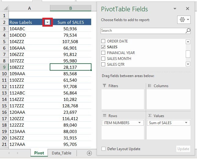
This is our current Pivot Table setup. We will be filtering the ITEM NUMBERS alphanumeric values. They come in the format of 3 numbers followed by 3 letters (e.g. 123ABC):

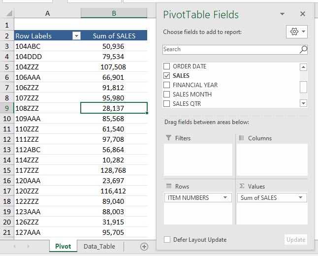
STEP 1: Click on the Row Label filter button in the Pivot Table.

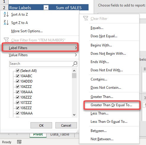
STEP 2: Select Label Filters.

You will see that we have a lot of filtering options. Let us try out – Greater Than Or Equal To

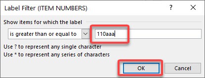
STEP 3: Type in 110aaa to get the values 110aaa and below when sorted alphabetically. You can see that the Label Filter will be applied to the ITEM NUMBERS.

Click OK.

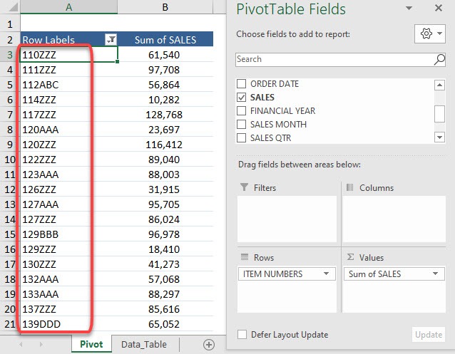
Now we have the filtering applied in a flash!

You can see the values 110ZZZ, 120AAA, 139DDD are there as they are greater than or equal to 110AAA. It is impressive that filtering can be done to the alphanumeric text.

You can also use Pivot Table to filter Top/Bottom items by value or percentage, etc, filter greater than or less than values, etc. Click here to learn all about Pivot Tables.

Make sure to download our FREE PDF on the 333 Excel keyboard Shortcuts here:

Bryan

Bryan Hong is an IT Software Developer for more than 10 years and has the following certifications: Microsoft Certified Professional Developer (MCPD): Web Developer, Microsoft Certified Technology Specialist (MCTS): Windows Applications, Microsoft Certified Systems Engineer (MCSE) and Microsoft Certified Systems Administrator (MCSA).

He is also an Amazon #1 bestselling author of 4 Microsoft Excel books and a teacher of Microsoft Excel & Office at the MyExecelOnline Academy Online Course.