Group By Custom Dates With Excel Pivot Tables

In my previous Group By Month post, we grouped our Sales by each month. However the cool thing with Excel is that we can take that a step further and customize our grouped date range!

Key Takeaways

• Group Dates for Better Analysis – Pivot Tables let you group dates by day, month, quarter, or year to uncover trends more easily.

• Manual Grouping for Custom Ranges – You can manually group specific date ranges (e.g., weeks, fiscal periods) by selecting and grouping them.

• Right-Click to Access Grouping – Simply right-click a date cell in the Pivot Table and choose Group to begin customizing your grouping.

• Ungroup if Needed – You can ungroup any custom date groups to reset back to individual dates by right-clicking and selecting Ungroup.

• Use Helper Columns for Complex Custom Groups – When built-in grouping doesn’t meet your needs, use a helper column in the source data to define custom date labels.

How to Group By Custom Dates With Excel Pivot Tables

In the example below I show you how to get the Sales Grouped by Custom Dates:

STEP 1: Insert a new Pivot table by clicking on your data and going to Insert > Pivot Table > New Worksheet or Existing Worksheet

 

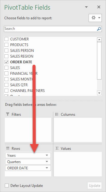
STEP 2: In the ROWS section put in the Order Date field.

Notice that in Excel 2016 (the version that I am using) it will automatically Group the Order Date into Years & Quarters:

 

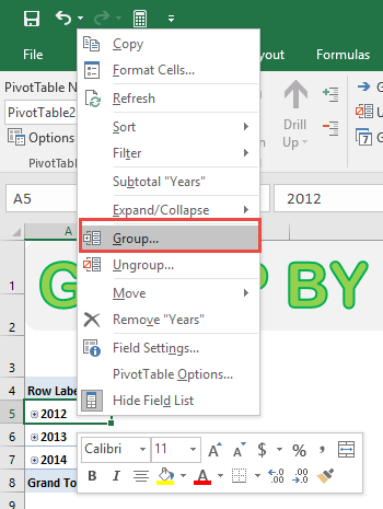
STEP 3: Right click on any row in your Pivot Table and select Group so we can select our Group order that we want:

 

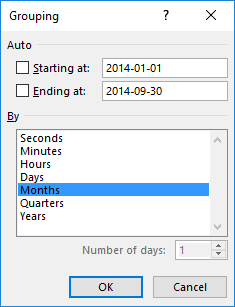
STEP 4: We need to deselect Quarters, Years and make sure only Months are selected (which will be highlighted in blue). This will group our dates by the Months only.

We can now define a custom date range!

For example, we can only show the Sales numbers from January 2014 to September 2014.  To do this we need to set the following:

Starting at: 2014-01-01

Ending at: 2014-09-30

Click OK.

 

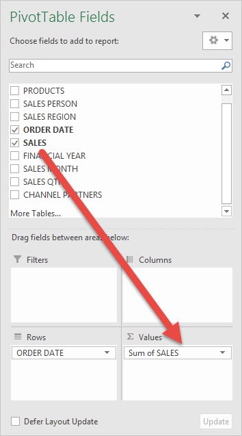
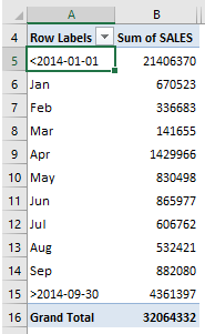
STEP 5: In the VALUES area put in the Sales field.  This will show the total of the Sales for each Month:

 

We can see that everything that does not fall in between January and September is Grouped into its own bucket.

 

STEP 6: Now we have our sales numbers grouped by Month & Years, notice that we can improve the formatting.

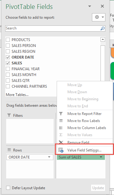
Click the Sum of SALES and select Value Field Settings

 

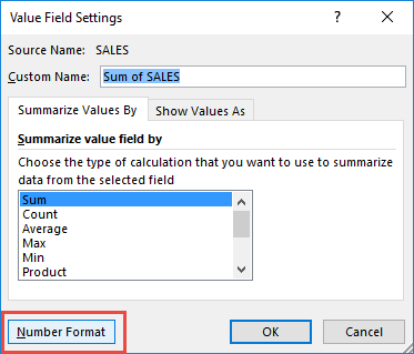
STEP 7: Select Number Format

 

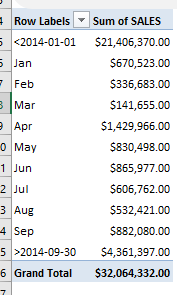
STEP 8: Select Currency. Click OK.

You now have your total sales for each monthly period based on your custom dates! Very Easy!

Frequently Asked Questions

How do I group dates in a Pivot Table by month and year?
Right-click on a date in your Pivot Table, click Group, then select both Months and Years in the dialog box.

Can I create my own custom date groups, like fiscal quarters?
Yes, use a helper column in your source data that defines the fiscal period, then use that column in your Pivot Table.

Why is the Group option greyed out?
This usually happens if your source data has blank cells or text instead of dates. Clean your data first to enable grouping.

Can I group by week in a Pivot Table?
Yes. When you group by Days, enter “7” in the Number of days field to group by weekly intervals.

What happens if I ungroup a grouped date field?
Excel will return your Pivot Table to show each individual date instead of the grouped range you previously set.