Learn the New Functions in Excel 2024: GROUPBY, PIVOTBY & IMAGE

Welcome to a groundbreaking era in Excel’s evolution with the introduction of Microsoft Excel 2024, featuring the revolutionary GROUPBY, PIVOTBY, and IMAGE functions. These additions are transforming data analysis, offering unprecedented control and creativity in managing, summarizing, and visualizing data. This suite of advanced functions is changing the game, making data more dynamic, insightful, and visually compelling than ever before.

Key Takeaways

1. GROUPBY and PIVOTBY streamline data summarization, enabling sophisticated manipulation and real-time insights directly within Excel, potentially reducing reliance on traditional pivot tables.
2. The IMAGE function integrates visual data representation within cells, adding a new dimension to data storytelling and analysis, allowing for more engaging and informative spreadsheets.
3. These functions simplify complex data arrangements, making it easier to group, aggregate, sort, and filter large datasets with precision and efficiency.
4. GROUPBY, in particular, offers automated updates that keep your summaries in sync with original data, ensuring your analysis remains current without manual intervention.

 

Introduction to Excel 2024’s Power Trio

The Age of Advanced Excel Functions

Welcome to the new era of data manipulation and reporting! Microsoft’s Excel 2024 introduces a game-changing set of features – the GROUPBY, PIVOTBY, and IMAGE functions, which will reshape your data analysis experience. These functions are not just enhancements; they are revolutionary tools that offer you the power to handle data in ways previously unimaginable in Excel.

How GROUPBY, PIVOTBY & IMAGE Revolutionize Data Analysis

Gone are the days of cumbersome data arrangements and static analysis. With Excel 2024, the GROUPBY and PIVOTBY functions are setting the stage for dynamic and sophisticated data manipulation. They make summarizing and reorganizing data so intuitive that you might find yourself saying goodbye to traditional pivot tables.

Picture this: GROUPBY automatically updates and maintains sync with your original data, delivering real-time insights with ease. Moreover, PIVOTBY allows for a horizontal layout, which is a breeze when it comes to comparing different categories side by side.

To add an extra layer of allure, the IMAGE function brings the power of visuals right into your cells. This means your data won’t just tell the story; it will show it with vivid images that update dynamically. The synergy between these functions is not just an improvement; it’s a revolution in Excel-based data analysis.

 

Exploring the GROUPBY Function

Simplified Grouping for Enhanced Insights

GROUPBY is your new ally in Excel for streamlining complex datasets into meaningful summaries. With its straightforward functionality, you can quickly condense rows of data based on shared characteristics, giving you at-a-glance insights. Imagine simply deciding the criteria, and Excel does the rest, grouping your data with refined efficiency.

The GROUPBY function in Excel is designed to group rows that contain the same values in specified fields and then perform calculations like sum, average, count, etc., on those groups. It’s particularly useful when working with large datasets that require aggregation based on certain criteria.

The syntax of this function is –

=GROUPBY(row_fields, values, function, [field_headers], [total_depth], [sort_order], [filter_array])

• row_fields: The range or array of rows you want to group.
• values: The range or array that contains the values you want to aggregate.
• function: The aggregation function to use on the values. This can be sum, average, count, etc.
• field_headers (Optional): Specifies whether the row_fields and values have headers and whether field headers should be returned in the results. The values could be:
  • 0 – No,
  • 1 – Yes and don’t show,
  • 2 – No but generate
  • 3 – Yes and show.
• total_depth (Optional): Determines whether the row headers should contain totals. The possible values could be:
  • 0 – No Totals
  • 1 – Grand Totals
  • 2 – Grand and Subtotals
  • -1 – Grand Totals at Top
  • -2 – Grand and Subtotals at Top.
• sort_order (Optional): Specifies the sequence of columns to sort by, starting with those in row_fields and then proceeding to the columns in values. A negative number signifies that the sorting of rows will be in a descending or reverse sequence.
• filter_array (Optional): A column-oriented 1D array of Booleans that indicate whether the corresponding row of data should be considered.

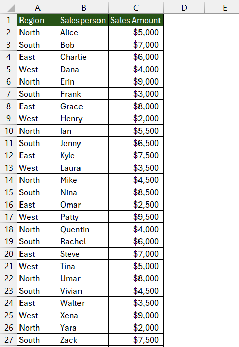
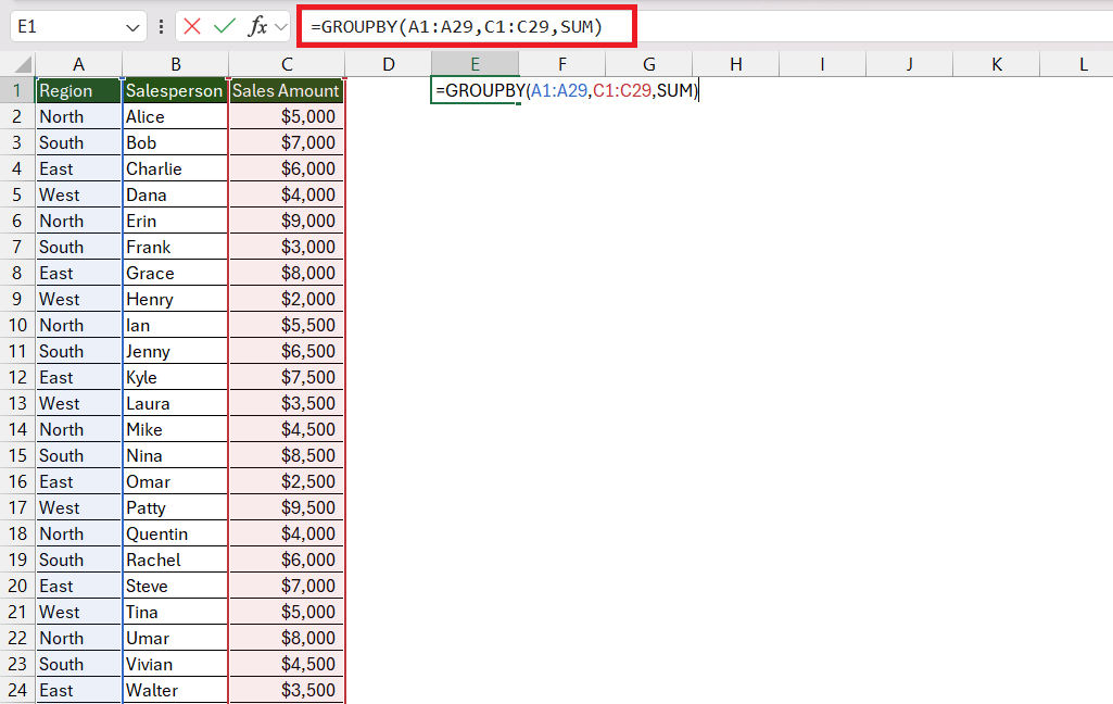
Here’s a direct example: Imagine you have a dataset with sales information, including Salesperson, Region, and Sales Amount. You want to group the data by Region, summing up the Sales Amount for each region.

Assuming your data is in the range A2:C29, where A2:A29 contains Region, B2:B29 contains Salesperson, and C2:C29 contains Sales Amount, the GROUPBY function might look like this:

Follow the steps below to achieve this –

STEP 1: Prepare Data: Identify the dataset you wish to group and aggregate.

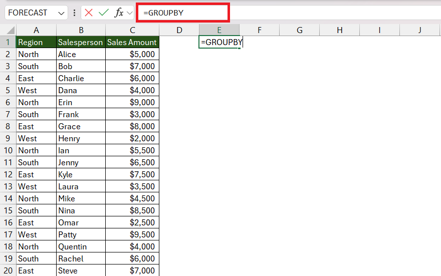
STEP 2: Enter the GROUPBY function.

=GROUPBY

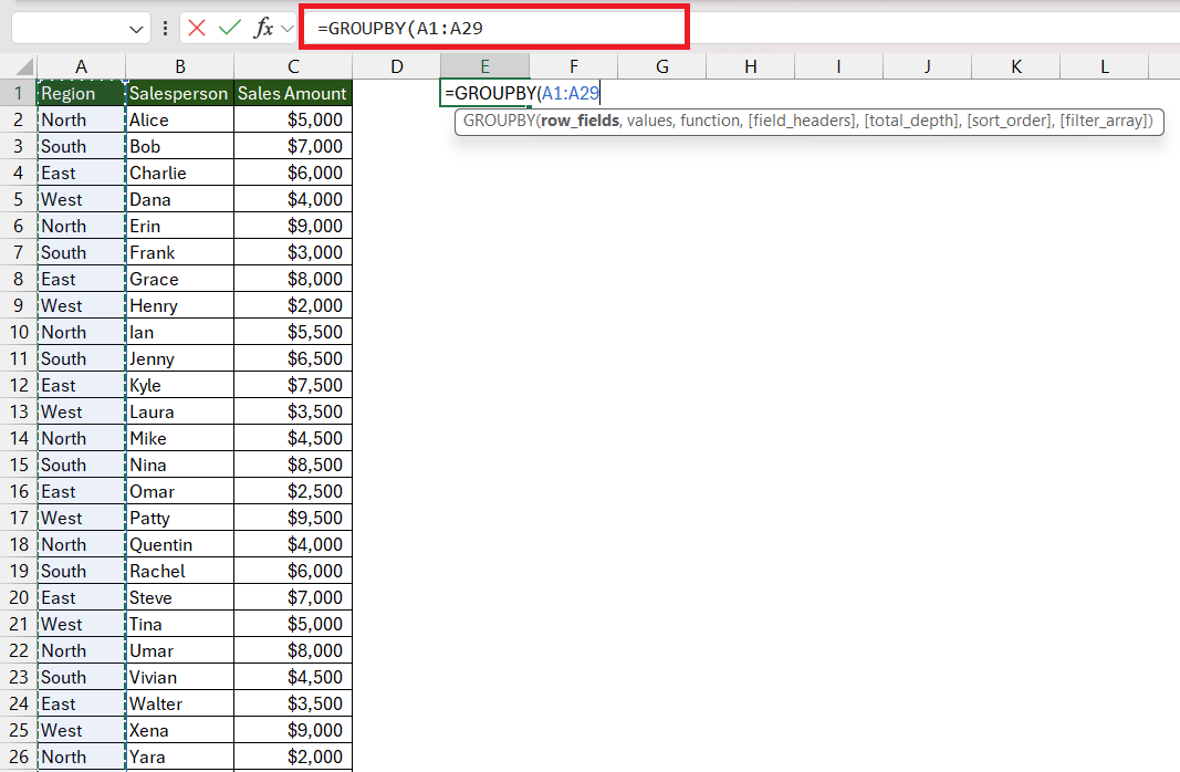
STEP 3: Define Grouping: Choose the columns (row_fields) by which you want to group your dataset.

=GROUPBY(A1:A29

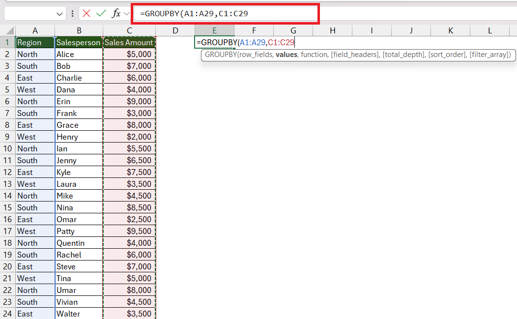
STEP 4: Select Values to Aggregate: Specify the range of values (values) over which to perform the aggregation function.

=GROUPBY(A1:A29,C1:C29

STEP 5: Choose Aggregation Function: Decide on the function (function) to apply to each group, such as sum, average, or count.

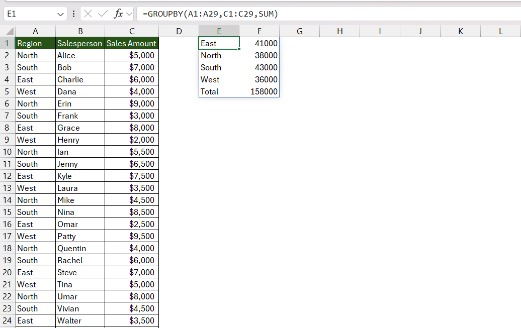
=GROUPBY(A1:A29,C1:C29,SUM)

Apply Optional Parameters: If necessary, set field headers, total depth, sort order, and a filter array to refine your grouping and aggregation.

STEP 6: Write the GROUPBY Function: Enter the function in a cell to operate.

Engage GROUPBY to hastily produce a summary of sales. You just pick your sales data and GROUPBY does the heavy lifting, kindly handing you a neatly organized table. Not only does this save time, but it also opens doors for sharper decision-making based on the unveiled trends.

 

Creative Uses of GROUPBY in Real-World Scenarios

Embrace creativity with GROUPBY, going beyond the basics to tailor unique solutions in everyday scenarios. For instance, imagine grouping customer feedback by sentiment to quickly address issues, or summarizing incident reports by cause in a safety dashboard.

GROUPBY’s versatility shines when sales data reveal the most profitable products or when HR departments assess staff performance across different company branches.

Real-World Scenario: Inventory Management

• GROUPBY can quantify stock levels by product type, enabling businesses to optimize their inventory and reduce costs more efficiently.

Marketing Campaign Analysis

• Apply GROUPBY to dissect campaign data by demographic, helping to pinpoint where marketing efforts resonate the most and tailor strategies accordingly.

These are merely glimpses of GROUPBY’s potential, bestowing you with the power to customize data in ways that resonate most for your specific context.

 

Mastering the PIVOTBY Feature

Define PIVOTBY with syntax

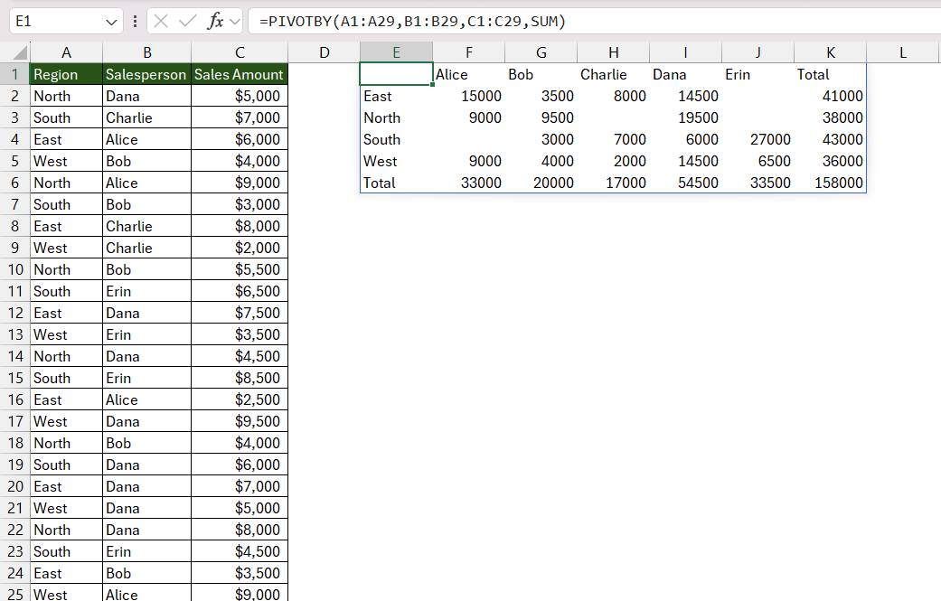
The PIVOTBY function in Excel enables you to efficiently organize, summarize, arrange, and refine your dataset according to specified row and column criteria.

Here’s the syntax –

=PIVOTBY(row_fields, col_fields, values, function, [field_headers], [row_total_depth], [row_sort_order], [col_total_depth], [col_sort_order], [filter_array])

• row_fields: The column(s) designated to appear as rows within the report.
• col_fields: The column(s) set to spread across the columns of the report.
• values: The column(s) selected for aggregation, serving as the data values in the report.
• function: The method of aggregation applied to the values, such as SUM, AVERAGE, etc.
• field_headers (Optional): Specifies whether the row_fields and values have headers and whether field headers should be returned in the results. The values could be:
  • 0 – No,
  • 1 – Yes and don’t show,
  • 2 – No but generate
  • 3 – Yes and show.
• row_total_depth(Optional): Determines whether the row headers should contain totals. The possible values could be:
  • 0 – No Totals
  • 1 – Grand Totals
  • 2 – Grand and Subtotals
  • -1 – Grand Totals at Top
  • -2 – Grand and Subtotals at Top.
• row_sort_order (Optional): Directs the sorting of rows based on specified criteria. Positive or negative numbers dictate the sorting order and direction, referencing columns in row_fields and values.
• col_total_depth (Optional): Similar to row_total_depth, this determines the inclusion and placement of total columns, with options for no totals, grand totals, and subtotals.
• col_sort_order(Optional): Governs column sorting in a manner similar to row_sort_order, with positive or negative numbers indicating sort order and direction, referencing columns in col_fields and values.
• filter_array (Optional): A one-dimensional array of Boolean values that filter the data, including or excluding rows based on true or false values.

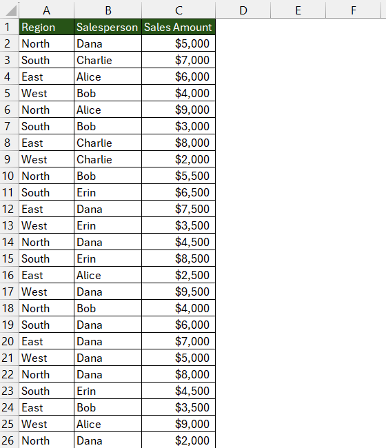
Follow the steps below to use PIVOTBY function in Excel –

STEP 1: Prepare Data: Identify the dataset you wish to group and aggregate.

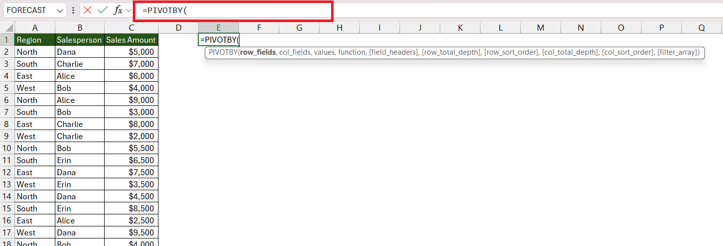
STEP 2: Enter the PIVOTBY function.

=PIVOTBY

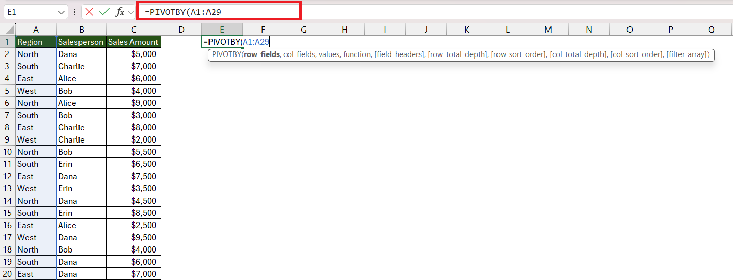
STEP 3: Select the range to appear as rows within the report.

=PIVOTBY(A1:A29

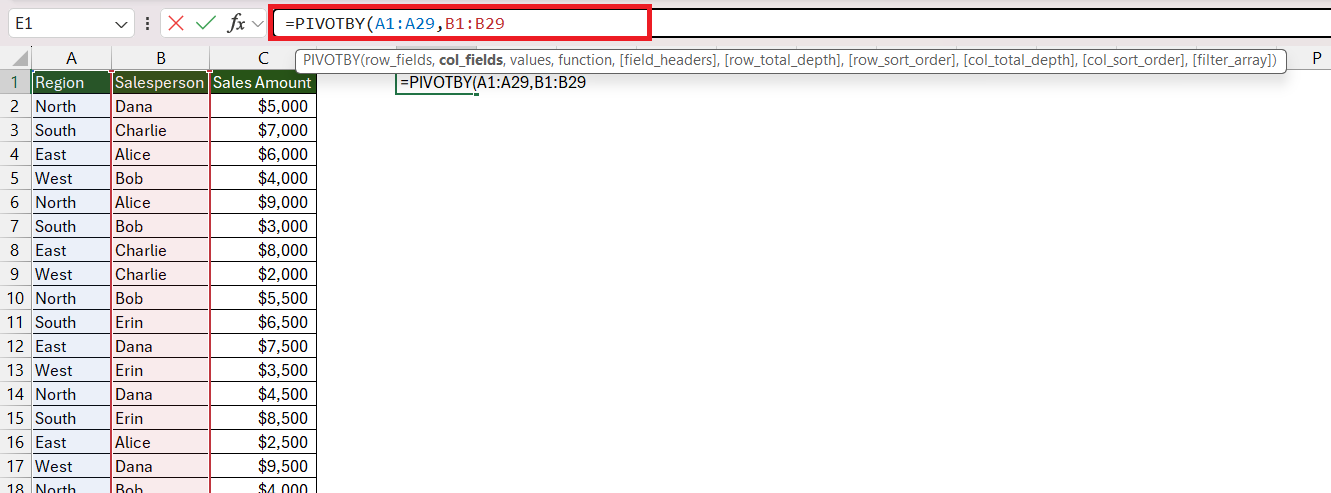
STEP 4: Select the range to appear as columns within the report.

=PIVOTBY(A1:A29,B1:B29

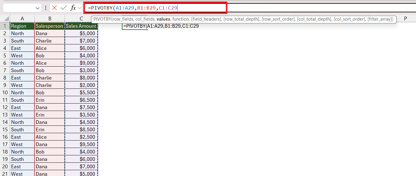
STEP 5: Select the range to appear as values within the report.

=PIVOTBY(A1:A29,B1:B29,C1:C29

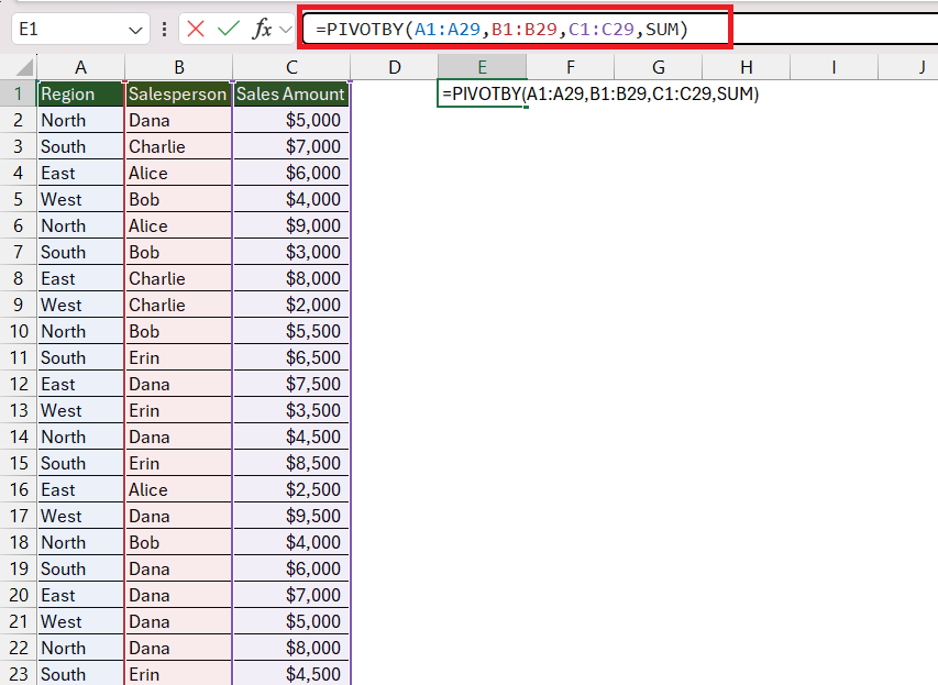
STEP 6: Decide on the function (function) to apply to each group, such as sum, average, or count.

=PIVOTBY(A1:A29,B1:B29,,C1:C29,SUM)

Apply Optional Parameters: If necessary, set field headers, total depth, sort order, and a filter array to refine your grouping and aggregation.

STEP 7: Enter the function in a cell to operate.

 

PIVOTBY vs. Traditional PivotTables

When it comes to organizing your data in Excel, PIVOTBY and traditional PivotTables both serve the purpose of summarizing and analyzing, but they’re not quite the same. While PivotTables have been the go-to for years, PIVOTBY is the newcomer with a fresh take.

PIVOTBY Advantages:

• It’s formula-based, which means your summaries can dynamically update right within your spreadsheet grid—no more manual refresh!
• It embraces multi-dimensional layouts, giving you the power to cross-tabulate data with minimal fuss.

Traditional PivotTables Strengths:

• They thrive with large datasets, effortlessly managing and summarizing without importing everything into the grid.
• PivotTables are champions of multiple aggregations—summing, averaging, counting—all neatly packaged in one place.
• They also carry the torch of compatibility; your PivotTable-heavy workbooks will play nice with all Excel versions.

Remember, each function has its strengths—PIVOTBY for its modern, dynamic nature, and PivotTables for their robust handling of big data and ubiquity across Excel editions.

Choosing between the two often depends on the specific needs of your project and the Excel version at play. PIVOTBY, with Microsoft 365, could streamline your workflow, but if you’re working with a mix of Excel environments, PivotTables still have an important role.

 

The Magic of Excel’s IMAGE Function

Inserting and Managing Images within Cells

With Excel’s IMAGE function, inserting and managing images within cells becomes a task as simple as any other data entry. This function breathes life into your spreadsheets, enabling them to be more visual and informative, perfect for dashboards, catalogs, or just adding context to your data.

To insert images, use the =IMAGE(“URL”) formula, which allows you to reference images by their URLs directly.

You can resize and adjust these as needed – making the aesthetics of your data presentation as flexible as your analysis.

For image management:

• Keep your images organized by ensuring their URLs are readily available within your dataset.
• Utilize Excel’s cell formatting options to maintain a consistent look and feel.

The practicality extends to businesses that need to manage product inventories with images or analysts creating visually rich reports. Excel now lets you view the bigger picture, quite literally, through the lens of your data.

 

Dynamic Image Functions for Visual Data Representation

Imagine adding a layer of visual storytelling to your dense spreadsheets. The IMAGE function does just that by injecting dynamic, context-rich imagery into Excel cells. This serves not only to beautify your data but also to streamline processes like comparisons and identification, allowing for quicker and more intuitive data analysis.

This function doesn’t just place a static picture; it opens avenues for images to be as dynamic as the data themselves. When the data changes or updates, so too can the linked images, keeping all information synchronized. This ensures your reports are always up to date, providing a living document that reflects the current state with accuracy and clarity.

Dynamic uses of the IMAGE function could include:

• Updating product photos in an inventory based on stock numbers.
• Changing the images in a sales report to highlight top-performing products with visuals.
• Displaying company logos next to financial data for quick brand recognition.

With these advancements, your documents can become interactive and engaging, making the experience of navigating through Excel sheets both aesthetically pleasing and functionally superior.

 

Tips for Smooth Function Combination in Complex Projects

Combining functions like GROUPBY, PIVOTBY, and IMAGE in complex Excel projects may seem daunting, but a few tips can streamline the process:

1. Plan Before You Implement: Outline your data structure and decide on how these functions can best serve your objectives.
2. Keep It Consistent: Use consistent naming conventions and data formatting to ensure your functions work seamlessly together.
3. Test in Phases: Implement and test each function individually before combining them to troubleshoot issues more effectively.
4. Document Everything: Comment your formulas and maintain a log of changes, especially when working in a team setting.
5. Optimize for Performance: Large datasets may impact performance, so consider using Excel tables or optimizing your formulas for speed.

By following these tips, you can tackle complex Excel projects with confidence, knowing that your GROUPBY, PIVOTBY, and IMAGE functions will work harmoniously to deliver powerful insights.

Remember to leverage Excel’s help resources or reach out to the vibrant online community for advice if you encounter any stumbling blocks. Excel professionals are often eager to share their expertise and may provide the nugget of wisdom that makes all the difference in your project.

 

FAQs: Unveiling More Secrets of GROUPBY, PIVOTBY & IMAGE

Can You Link GROUPBY & PIVOTBY Results to Other Excel Features?

Absolutely, you can link results from GROUPBY & PIVOTBY to other Excel features for a more dynamic and integrated experience. Whether it’s charts, conditional formatting, or even other functions, these results are just like any other cell value in Excel and can be referenced throughout your workbook for extended analysis.

What Are the Common Challenges When Using the IMAGE Function?

Some common challenges with the IMAGE function include images not displaying if they are not hosted online or if authentication is required, difficulty in managing image sizes within cells, and static display of GIF files. It’s also not fully compatible across all Excel platforms, which can cause inconsistencies.

How does the groupby function work in excel?

The GROUPBY function in Excel helps you group rows of data based on common attributes and apply aggregate functions like SUM or AVERAGE to numerical data. You set the criteria for grouping within the formula, and Excel organizes the data accordingly, displaying the results in a new array.

What were the mean sales in this month, by salesperson?

To calculate the mean sales in a month by salesperson, you would use an AVERAGEIF or AVERAGEIFS function in Excel to average the sales amounts based on the specific salesperson and the month in question.

Why don’t I have the GROUPBY function in Excel?

If you don’t see the GROUPBY function in Excel, you may be using an older version of Excel that doesn’t support it. GROUPBY is introduced in Excel 365 and later versions. Ensure your application is updated to the latest version to access this function.