How to Combine VLOOKUP and IFERROR to Replace the #N/A Error in Excel

Ever tried to use the  VLOOKUP Function, but it returns a #N/A error? Do not worry, as it is very easy to fix this error when you combine VLOOKUP with IFERROR! This is one of the most common frustrations for Excel users. The good news is that it’s also one of the easiest to fix.

In this article, we’ll walk through why #N/A errors occur with VLOOKUP, and how to combine VLOOKUP with IFERROR to handle these errors gracefully.

Key Takeaways:

• VLOOKUP searches data vertically and returns a matching value from another column.
• #N/A errors occur when VLOOKUP cannot find the lookup value in the source table.
• IFERROR cleans up errors by replacing them with custom text, numbers, or blanks.
• Combining VLOOKUP with IFERROR makes reports professional and user-friendly.
• You can also use IFNA or ISNA as alternatives, but IFERROR is the simplest option.

I explain how you can do this below:

Introduction to VLOOKUP and IFERROR

What is VLOOKUP?

VLOOKUP stands for Vertical Lookup. It’s used to search for a value in the first column of a table and return a corresponding value from another column in the same row.

Syntax:

=VLOOKUP(lookup_value, table_array, col_index_num, [range_lookup])

• lookup_value → The value you want to search for.
• table_array → The range of data where you want to look.
• col_index_num → The column number (starting from 1) that contains the result you want.
• [range_lookup] → TRUE for approximate match, FALSE for exact match.

What is IFERROR?

IFERROR is an error-handling function. It tells Excel what to do if a formula results in an error (like #N/A, #DIV/0!, #VALUE!, etc.).

Syntax:

=IFERROR(value, value_if_error)

• value → The formula or calculation you want to evaluate.
• value_if_error → What to return if the formula results in an error.

Why Use IFERROR with VLOOKUP?

Here are some reasons you’ll want to combine these two functions:

• Professional Appearance – Dashboards and reports should never show cryptic Excel errors.
• Better User Experience – End-users immediately understand that the item is missing instead of seeing #N/A.
• Flexibility – You can replace errors with custom messages, numbers, or even blanks.
• Error Handling in Automation – If you’re preparing files for clients or management, you want automated handling of missing data.
• Prevents Broken Formulas from Distracting You – Errors stand out, but they can make your data harder to read if left untreated.

 

Combine VLOOKUP and IFERROR to Replace the #N/A Error

STEP 1: Let us use VLOOKUP to get the cost of the item:

=VLOOKUP(E6, $A$6:$C$8, 3, FALSE)

• E6 will give us the value to lookup (Tablet)
• $A$6:$C$8 will highlight the entire table of source data
• 3 as we want the Cost which is in the third column
• FALSE will ensure it’s an exact match

Apply the same formula to the rest of the cells by dragging the lower right corner downwards.

You will see there’s a #N/A value! 

That is because Lamp is not included in the source table.

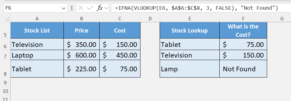
STEP 2: Let us make it look better with IFERROR!

If we wrap IFERROR around the VLOOKUP formula, it will replace these invalid values with the text that we specify, “Not Found“:

=IFERROR(VLOOKUP(E6, $A$6:$C$8, 3, FALSE), “Not Found”)

Apply the same formula to the rest of the cells by dragging the lower right corner downwards.

And just like that, you now have clean results!

 

Tips & Tricks

Alternatives to IFERROR

Excel has other functions for error handling, too:

• IFNA → Specifically replaces #N/A errors, while leaving other errors visible.

=IFNA(VLOOKUP(E6, $A$6:$C$8, 3, FALSE), “Not Found”)

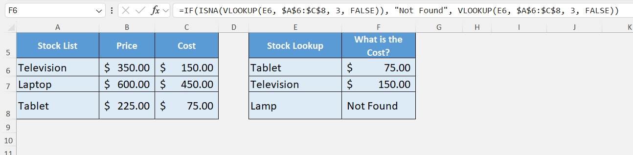
• ISNA with IF → An older way of doing the same thing.

=IF(ISNA(VLOOKUP(E6, $A$6:$C$8, 3, FALSE)), “Not Found”, VLOOKUP(E6, $A$6:$C$8, 3, FALSE))

IFERROR is still the most straightforward and widely used option.

Common Mistakes

• If you don’t lock your source table with dollar signs (e.g., $A$6:$C$8), dragging the formula down will break the range.
• While IFERROR cleans up your spreadsheet, don’t forget that the underlying data issue (missing values) is still real.
• Replacing errors with blanks can be visually nice, but it might cause trouble if you’re summing or averaging those cells later.
• Always set the fourth argument in VLOOKUP to FALSE unless you specifically want an approximate match. Otherwise, you might get incorrect results.

 

Practical Applications

Here are some real-world scenarios where this trick is a lifesaver:

• Sales Reports – Match customer IDs with sales data; if a customer is missing, show “Not Found” instead of errors.
• Inventory Management – Look up product availability; errors become “Out of Stock.”
• Finance Models – Replace errors with zero when doing revenue or cost lookups.
• Data Cleaning – Import data from external sources and handle missing matches smoothly.
• Dashboards – Keep your visualizations free from errors that might confuse stakeholders.

 

FAQs

1. Why does VLOOKUP return a #N/A error?

VLOOKUP formula returns a #N/A error when it cannot find the value you are searching for in the source table’s first column. This happens if the lookup value is misspelled, doesn’t exist in the table, or if you’ve set the wrong range. Sometimes, hidden spaces or formatting differences between the lookup value and the table data also cause the error. While technically correct, the error looks unprofessional in reports. That’s why using IFERROR to handle it is a smart choice.

2. How does IFERROR work in Excel?

IFERROR checks whether a formula results in an error and, if it does, returns an alternative result that you specify. It can handle a wide range of errors including #N/A, #DIV/0!, #VALUE!, and more. This makes it versatile for cleaning up messy outputs in complex spreadsheets. For example, =IFERROR(10/0, “Error Detected”) will return “Error Detected” instead of #DIV/0!. When used with VLOOKUP, it ensures your results look neat even when matches are missing.

3. What is the formula to combine VLOOKUP with IFERROR?

The standard formula is:

=IFERROR(VLOOKUP(lookup_value, table_array, col_index_num, FALSE), “Not Found”)

Here, VLOOKUP searches for the value, and if it’s found, it returns the result. If it’s missing, IFERROR steps in and replaces the error with “Not Found” (or any text, number, or blank you prefer). This ensures your table never shows #N/A, keeping everything clean. You can also replace errors with 0, empty strings, or a custom message like “Item not in list”.

4. What are common mistakes when using VLOOKUP and IFERROR?

One common mistake is not using absolute references (like $A$2:$C$10) in your source table range, which causes broken formulas when copied. Another mistake is replacing errors with blanks in financial models, which can mess up totals and averages. Users also sometimes set the range_lookup argument to TRUE accidentally, which allows approximate matches and can lead to incorrect results. Finally, relying only on IFERROR may hide underlying data issues instead of fixing them. Always use it thoughtfully.

5. Can I use alternatives to IFERROR with VLOOKUP?

Yes, Excel provides alternatives like IFNA and ISNA with IF. IFNA works just like IFERROR but only handles #N/A errors, leaving other errors visible. ISNA with IF is the older method, but it’s longer to write and less efficient. For example:

=IF(ISNA(VLOOKUP(E2, A2:C10, 2, FALSE)), “Not Found”, VLOOKUP(E2, A2:C10, 2, FALSE))

However, IFERROR remains the simplest and most widely used choice for error handling in modern Excel versions.