How to Use IF Function with Multiple Conditions in Excel

Logical functions in Microsoft Excel are like your trusted sidekicks, empowering you to make decisions and automate data analysis. Imagine navigating through vast data effortlessly with simple formulas—logical functions make that possible.

Key Takeaways:

• Understanding IF Function: Excel’s IF function directs data down different paths based on conditions, providing dynamic decision-making capabilities.
• Syntax Mastery: Learn the structure of an IF statement to effectively communicate with Excel, ensuring your formulas work as intended.
• Handling Multiple Conditions: Utilize AND and OR operators with IF to manage complex criteria, tailoring your data management to real-world scenarios.
• Inverting Logic with NOT: Incorporate the NOT function to reverse conditions, refining your data analysis to capture precise criteria.
• Advanced Techniques: Explore advanced techniques like combining IF with other functions, transitioning to IFS, and leveraging array formulas for bulk operations.

 

Introduction to Mastering the IF Function

The Power of Logical Functions in Excel

When you start to explore the tools that can make you an Excel superhero, logical functions are like your trusty sidekicks. These functions allow you to make decisions within your spreadsheets based on certain criteria, automating data analysis and making your worksheets interactive and responsive to changes. Imagine being able to sift through vast amounts of data with a few simple formulas—logical functions make that possible.

What Is the IF Function in Excel?

The IF function in Excel is akin to a digital crossroads, directing your data down one path or another based on conditions you set. At its core, it examines a particular condition and returns a value if that condition is true, and another value if it’s false.

Think of it as a fork in the road, where each path leads to a different outcome. This dynamic capability provides you with the power to make your spreadsheets work smarter, adapting to the data they contain in real time.

Understanding the Syntax of an IF Statement

Grasping the syntax of an IF statement is like understanding a new language’s basic grammar—it’s essential for you to communicate effectively with Excel. The IF function uses a logical test to check if something is true or false, and then it performs actions based on that test using the following structure: =IF(logical_test, value_if_true, value_if_false).

Each argument plays its part: the logical test is the condition you’re checking, the value_if_true is what you see if the condition is met, and the value_if_false is what appears if it’s not. It’s crucial to get this structure right to ensure your formulas work as intended.

 

Laying the Groundwork for Multiple Conditions

Single vs. Multiple Conditional Logic

Dealing with a single condition in an IF function is relatively straightforward—like deciding if an apple is red or not. But often, real-world data analysis isn’t that simple. Multiple conditional logic comes into play when you need to consider several factors at once, like checking if an apple is red, big, and sweet all together.

In Excel, this is where the AND and OR functions team up with IF, allowing you to set up complex criteria and have your spreadsheet respond accordingly. It’s a powerful way to tailor your data management to the nuanced scenarios you encounter.

Enhancing Decision-Making with AND & OR Operators

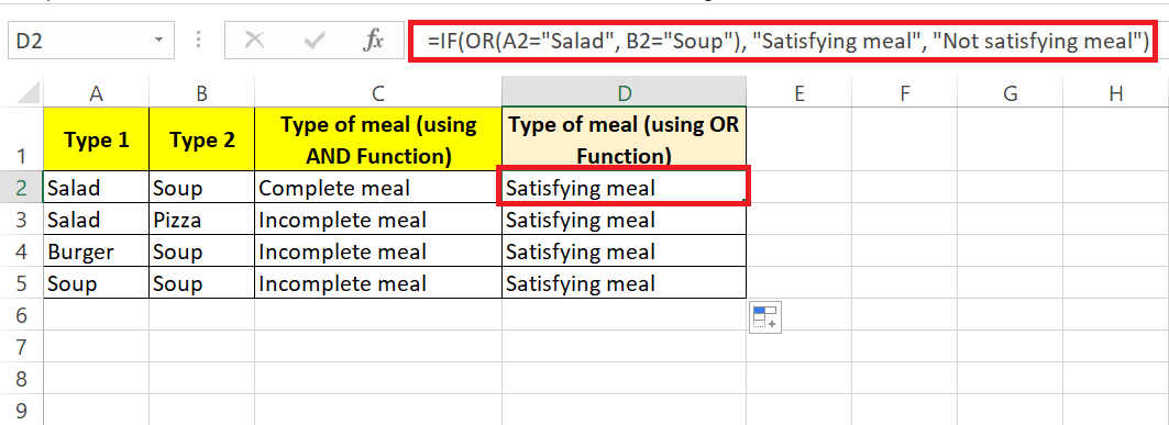
Imagine you’re at a buffet and you need to choose your meal. The AND operator is like requiring that your plate must contain both salad AND soup for it to be complete, whereas the OR operator is more lenient, allowing for either salad OR soup or perhaps both, for a satisfying meal. In Excel, the AND & OR operators amplify your decision-making power within IF statements by letting you set multiple criteria.

AND insists that all conditions be met, while OR is happy if any one condition is true. By using these operators, you can fine-tune your IF functions to handle complex, real-world data scenarios with ease.

Here’s an example IF function with AND and OR operators in Excel:

Identify the criteria for a complete or satisfying meal. Use the IF function with the AND or OR operator to define the conditions.

Here’s the scenario with the AND operator:

=IF(AND(A2=”Salad”, B2=”Soup”), “Complete meal”, “Incomplete meal”)

This formula checks if both Salad and Soup are selected. If so, it returns “Complete meal”; otherwise, it returns “Incomplete meal”.

Here’s the same scenario with the OR operator:

=IF(OR(A2=”Salad”, B2=”Soup”), “Satisfying meal”, “Not satisfying meal”)

This formula checks if either Salad or Soup (or both) are selected. If so, it returns “Satisfying meal”; otherwise, it returns “Not satisfying meal”.

Incorporating NOT for Reversed Logic

Every now and then, you find yourself needing to flip the script, and this is precisely where the NOT function becomes your ally in Excel. The NOT function is the contrarian that takes whatever condition you’ve given it and inverts it, turning what’s true to false, and vice versa.

It’s perfect for when you want to exclude certain data points or focus on the opposite of a given condition within your IF statements. By using NOT, you refine your data analysis, ensuring that you’re capturing precisely the conditions that matter to your unique situation.

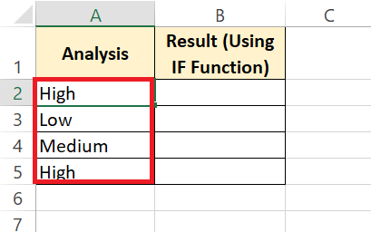
STEP 1: Identify the condition you want to reverse, such as checking if values are not “High”.

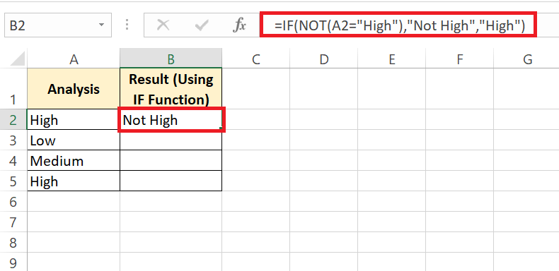
STEP 2: Use the NOT function to invert the condition, like NOT(A2=”High”). Apply the IF function to return “Not High” if the condition is true, otherwise “High”.

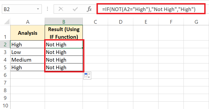
=IF(NOT(A2=”High”), “Not High”, “High”)

This formula checks if the value in cell A2 is not “High”. If it’s not “High”, it returns “Not High”; otherwise, it returns “High”.

STEP 3: Drag the formula to the rest of the cells. Review the results to ensure the inversion accurately reflects the desired logic.

 

Integrating IF with Other Powerful Excel Functions

Combining COUNTIF with IF

Juggling employee attendance records can be like assembling a complex puzzle. Each piece represents an employee’s daily presence, absence, or any special notes on their record. Excel equips you with the ability to use IF statements to dissect this information, enabling you to categorize employees based on their attendance patterns.

Multiple conditions within your IF formulas can quickly calculate perfect attendance bonuses, flag chronic absenteeism, or monitor adherence to company policies. Such detailed management is crucial for maintaining a fair and productive workplace.

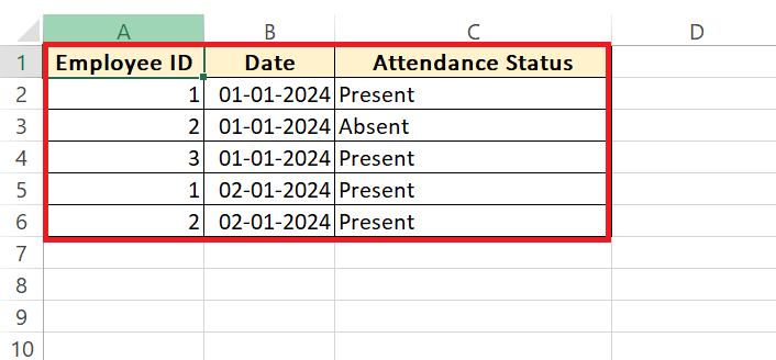
STEP 1: Set up your worksheet: Input your attendance data into Excel, organizing it with columns for Employee ID, Date, and Attendance Status.

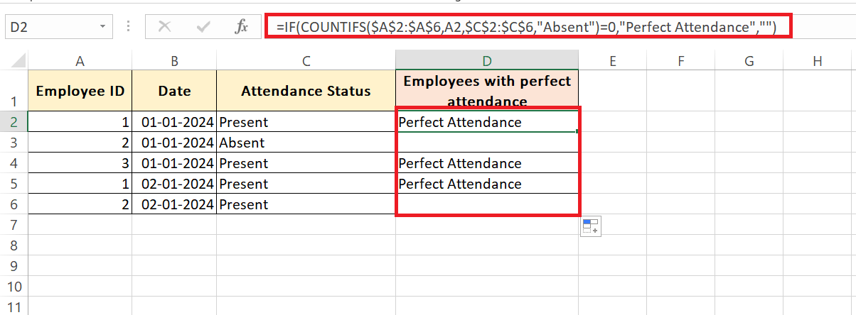
STEP 2: Create your IF statements: Suppose you want to identify employees with perfect attendance (present every day). In cell D2, enter:

=IF(COUNTIFS($A$2:$A$6,A2,$C$2:$C$6,”Absent”)=0,”Perfect Attendance”,””)

This formula counts the number of “Absent” instances for each employee and returns “Perfect Attendance” if the count is zero.

STEP 3: Drag the formula down: Drag the formula down to apply it to all employees in the dataset. This will categorize each employee based on their attendance pattern. Review the results to identify employees with perfect attendance or any other attendance patterns of interest.

You can use additional IF statements to further categorize employees based on different criteria.

Handling Errors Gracefully with IF and IS Functions

Imagine your spreadsheet as a high-speed train; errors are like obstacles on the track that can bring everything to a screeching halt. But with a clever conductor—IF combined with IS functions—the journey can continue smoothly, even when potential problems arise.

Use IFERROR to steer around common errors, returning a value you specify instead of Excel’s default error messages. IFNA is specifically tailored to deal with the notorious #N/A error. These error-handling functions help you maintain a clean and professional look to your work, keeping your data analysis credible and clear.

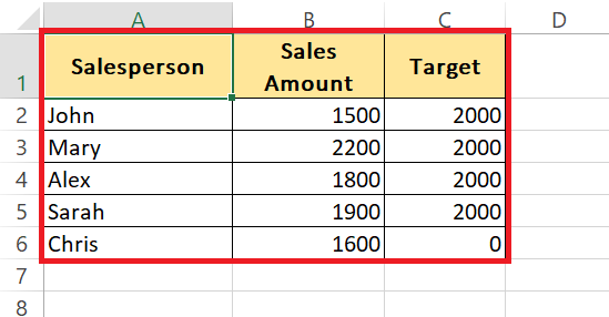
Let’s say we have a dataset containing sales data and we want to calculate the commission for each salesperson. However, some salespeople may not have achieved their sales target, resulting in a potential division by zero error. We can use the IFERROR function along with IF and IS functions to handle this error gracefully.

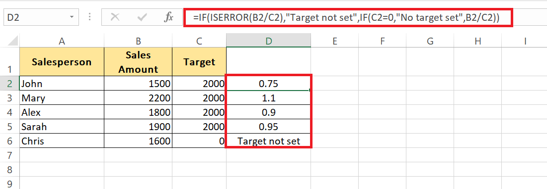
In cell D2, enter the following formula

=IF(ISERROR(B2/C2), “Target not set”, IF(C2=0, “No target set”, B2/C2))

This formula checks for two potential errors:

Division by zero (denominator is zero) and other errors. If there’s a division by zero error, it returns “No target set”. If there’s any other error, it returns “Target not set”.

Otherwise, it calculates the commission by dividing the sales amount by the target.

This way, even if there are errors in the data, the spreadsheet will display meaningful messages instead of default error messages, ensuring a smoother data analysis process.

 

Excel’s IFS Function – Simplifying Multiple Conditions

Breaking Down the IFS Function

Excel’s IFS function is like having a highly efficient traffic control system at a busy intersection—streamlining the process and keeping things moving smoothly. It allows you to test multiple conditions, one after the other, and when the first TRUE condition is found, it will return the corresponding value.

With IFS, there’s no need to nest IF statements inside one another, which simplifies the readability and maintenance of your workbook. It requires a series of pairs of conditions and values: =IFS(condition1, value1, condition2, value2, ...). As soon as it hits the first true condition, it acts on it, delivering streamlined logic and cleaner formulas.

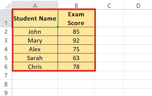
STEP 1: Set up your worksheet: Enter students’ names in column A and their respective exam scores in column B.

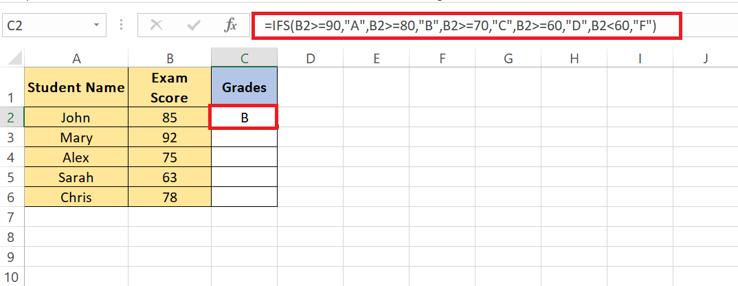
STEP 2: Apply the IFS function: In cell C2, enter the following formula:

=IFS(B2>=90, “A”, B2>=80, “B”, B2>=70, “C”, B2>=60, “D”, B2<60, “F”)

This formula checks the exam score in cell B2 against multiple conditions.

• If the score is 90 or above, it returns “A”.
• If the score is between 80 and 89, it returns “B”, and so on.

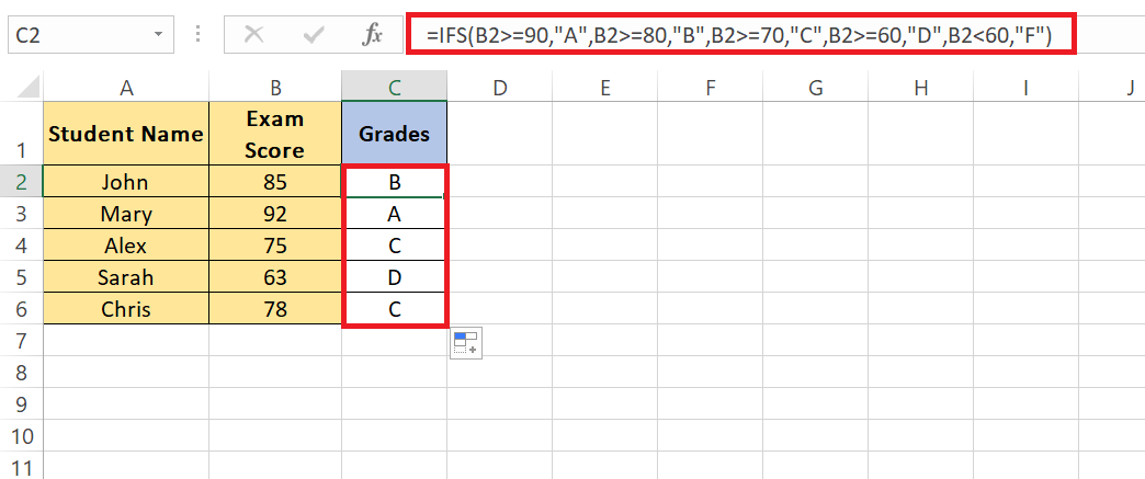
STEP 3: Drag the formula down: Drag the formula down for all students in the dataset. This will categorize each student’s exam score into their corresponding grade level.

This approach streamlines the process of grading students’ exam scores, making the logic clearer and the formulas easier to maintain.

Transitioning from Nested IFs to IFS

Moving from nested IFs to the sleeker IFS function is like trading a box of tangled cords for a wireless setup—it’s a liberating upgrade. The transition to IFS simplifies your formulas, reducing the chances of error and making your logic crystal clear.

Whereas nested IFs require you to keep track of each condition and its corresponding outcome within a hierarchy, IFS places each condition on equal footing, sequentially checking them without the hassle of managing multiple layers. If you’re working with the latest version of Excel that supports IFS, embracing this transition can save you time and mental bandwidth, producing more straightforward, cleaner worksheets.

 

Advanced Techniques for the Excel Pro

Leveraging Array Formulas with IF for Bulk Operations

Array formulas, teamed with the IF function, are like a superhero squad for your data processing, taking on bulk calculations with a single, sweeping formula. They enable you to perform multiple calculations across an array of cells and apply IF logic to a whole dataset at once. Imagine wanting to apply a discount to a batch of products based on varying conditions.

An array formula with IF could evaluate these conditions for every product simultaneously, determining the final price for each item in one fell swoop. This leap from individual cells to entire ranges boosts efficiency and consistency across your worksheet.

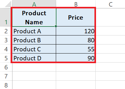
Suppose we have a dataset of product prices and we want to apply different discounts based on certain conditions using an array formula with IF.

STEP 1: Set up your worksheet: Enter the product names in column A and their respective prices in column B.

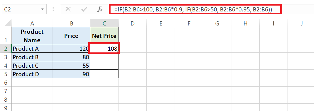
STEP 2: Apply the array formula with IF: In cell C2, enter the following array formula:

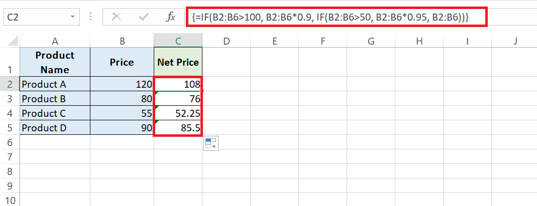
 =IF(B2:B6>100, B2:B6*0.9, IF(B2:B6>50, B2:B6*0.95, B2:B6)).

This formula evaluates multiple conditions simultaneously across the range of prices in column B. If a price is greater than 100, it applies a 10% discount. If it’s greater than 50 but less than or equal to 100, it applies a 5% discount.

Otherwise, it leaves the price unchanged.

STEP 3: Press Ctrl + Shift + Enter: Since this is an Excel Array Formulas Explainedarray formula, remember to press Ctrl + Shift + Enter instead of just Enter to apply it. Excel will then calculate the formula for each cell in the range, performing all calculations simultaneously.

This approach efficiently applies discounts to all products in the dataset based on their individual prices, enhancing productivity and consistency.

 

Conditional Formatting with IF Logic

Have you ever wanted your data to speak volumes at a glance? Conditional formatting powered by IF logic turns dull rows and columns into a vibrant dashboard, highlighting key information based on the rules you define.

You can set up conditional formatting to change cell colors, add icons, or even data bars, which all depend on IF statements to decide their appearance. Whether it’s to flag overdue tasks, celebrate achieved targets, or simply organize your data into an eye-catching and meaningful presentation, conditional formatting with IF logic transforms the way you, and others, interact with your data.

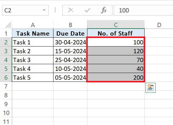
Let’s assume we have a dataset of task completion statuses where each row represents a task and each column represents different attributes such as Task Name, Due Date, Status, etc.

STEP 1: Select your data range: Highlight the range of cells you want to apply conditional formatting to in Excel.

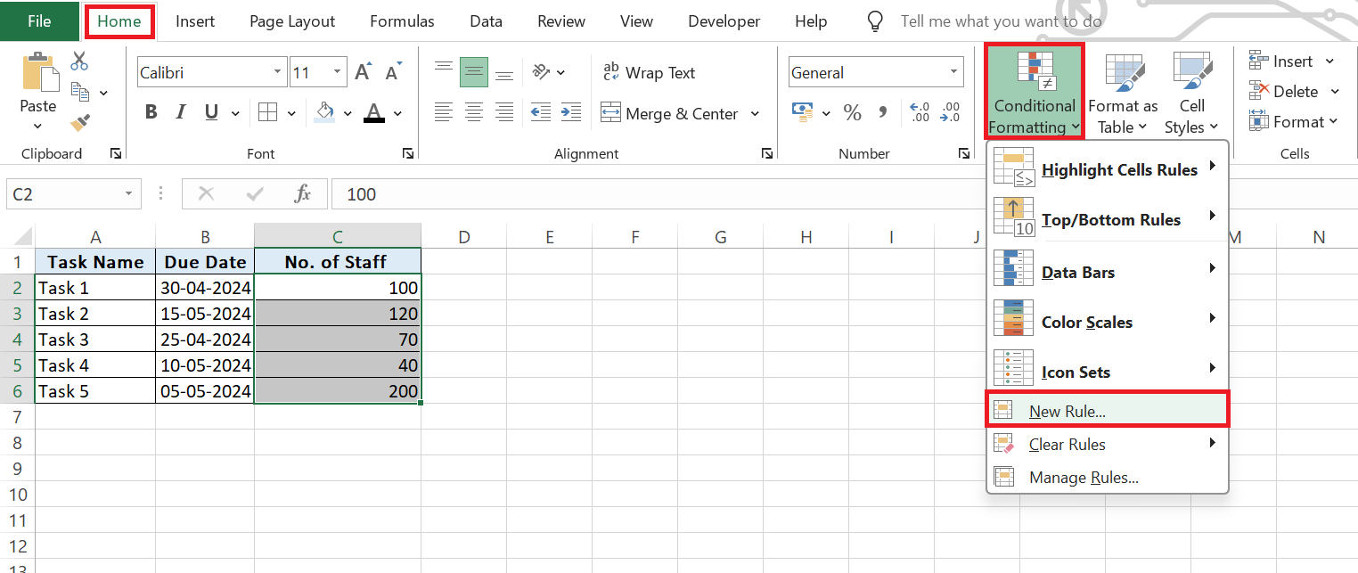
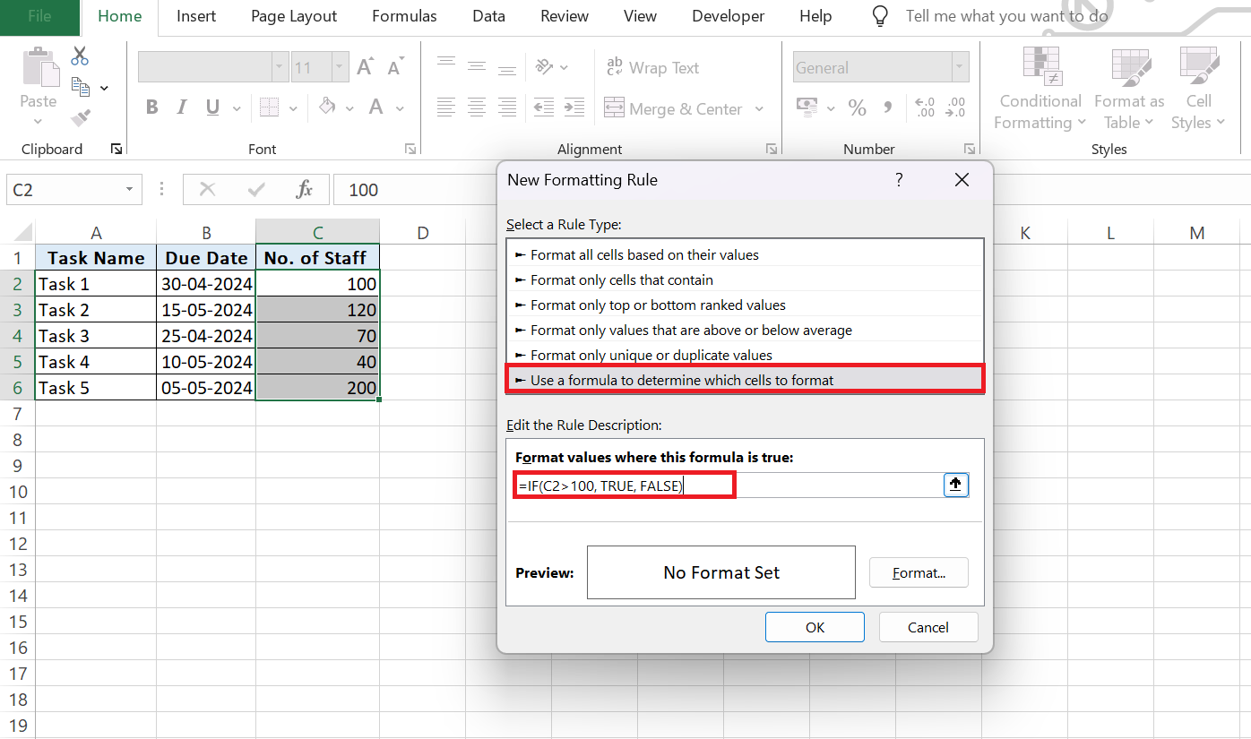
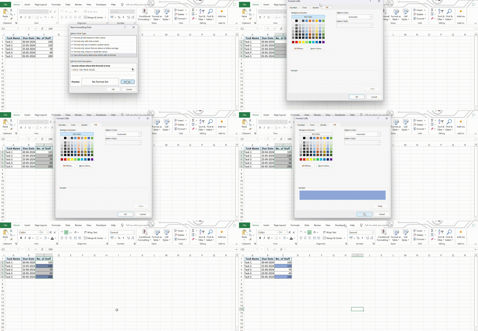
STEP 2: Go to Conditional Formatting: Navigate to the “Home” tab, click on “Conditional Formatting” in the ribbon, and choose “New Rule”.

STEP 3: Set up the rule: Select “Use a formula to determine which cells to format”, then enter your IF logic formula. For example, to highlight cells with values greater than 100, use a formula like “=IF(A1>100, TRUE, FALSE)”.

STEP 4: Choose formatting options: Specify the formatting style you want to apply when the condition is met, such as changing cell color or adding data bars. Click “OK” to apply the conditional formatting.

This dataset can be used to apply conditional formatting to highlight tasks that are overdue, in progress, completed, etc., based on the rules defined using IF logic.

 

Frequently Asked Questions

How Do I Write an IF Function with Three Conditions?

Crafting an IF function with three conditions involves a nested approach. Use the following syntax: =IF(condition1, value_if_true1, IF(condition2, value_if_true2, IF(condition3, value_if_true3, value_if_false3))). This allows you to check each condition in sequence, providing a value for each true condition, and a final outcome if all conditions are false. Remember to keep your logic structured and clear to avoid confusion.

Can You Have Too Many Nested IF Statements in Excel?

Indeed, you can have too many nested IF statements in Excel, which can lead to complex, hard-to-maintain formulas. Excel allows up to 64 nested IF functions, but it’s best to keep their number much lower. A high number of nested IFs can make formulas prone to errors and difficult to troubleshoot. Rather than jam-packing IF functions, consider alternative methods such as IFS, CHOOSE, or a combination of logical operations like AND and OR for greater efficiency and clarity.

How to use if function with 4 conditions in Excel?

Using an IF function with four conditions requires you to delve into further nesting or consider alternatives. For traditional nesting, structure it as =IF(condition1, value_if_true1, IF(condition2, value_if_true2, IF(condition3, value_if_true3, IF(condition4, value_if_true4, value_if_false4)))). For a less convoluted formula, Excel’s IFS function is ideal: =IFS(condition1, value1, condition2, value2, condition3, value3, condition4, value4), simplifying the logic by evaluating each condition in turn until it finds a TRUE one.

How do you write an if then formula in Excel?

Writing an ‘if then’ formula in Excel involves using the IF function, which checks a condition and returns a specified value if that condition is true. The basic syntax is =IF(logical_test, value_if_true, value_if_false). If the ‘logical_test’ (the condition) is met (‘then’), Excel returns ‘value_if_true’. Otherwise, it returns ‘value_if_false’.

How can one insert the if functions together with other microsoft excel functions?

Inserting IF functions together with other Excel functions is about weaving them into a single formula where IF acts as the decision-maker. For instance, to sum values only if they meet certain criteria, you could combine IF with SUM using a formula like =SUM(IF(logical_test, range_if_true, range_if_false)). Here, the IF function determines which values in the range are included in the SUM based on your logic. Always make sure to match the IF criteria with the appropriate function for the task at hand.