Excel is a potent and robust tool when working with an extensive dataset for calculation and analysis. However, it’s inevitable to encounter errors during such data processing. This is precisely where the IFERROR function in Excel proves to be helpful.
IFERROR function displays a custom message when a function’s output is an error.
In this article, we will be covering the following topics in detail –
Now, let’s explore each of these topics individually!
Download the Excel Workbook below to follow along and understand how to use the IFERROR function in Excel –
download excel workbookIFERROR-Function-in-Excel.xlsx
Introduction
The IFERROR function in Excel allows you to specify a value to be returned if a formula encounters an error. If you have a calculation that results in an error like, #N/A, #VALUE!, #REF!, #DIV/0!, #NUM!, #NAME?, then you can clean it up by using the IFERROR function which allows you to replace the error it with a 0 or a blank cell or a custom message.
The syntax of the IFERROR function in Excel is –
=IFERROR(value,value_if_error)
- value – The formula you want to evaluate.
- value_if_error – The value you want to display if the evaluated formula results in an error.
If the formula result is not an error, the function will simply display the formula’s result itself.
Types of Errors
Below are the different types of errors that you can face when working on Excel –
- #REF! – Excel will display #REF! error when the cell that is referenced in a formula does not exist or is invalid.
- #VALUE! – Excel displays an #VALUE! error when the variable provided in the formula is not a supported type.
- #DIV/0! – This error in Excel occurs when you attempt to divide a number with zero, any value equivalent to zero, or a blank cell.
- #NULL! – This error occurs when the range provided in the formula is not valid and you have provided an incorrect character instead of the required character in the range.
- #SPILL! – When the formula cannot populate all the cells it is supposed to, the first cell where the formula is entered shows the #SPILL! Error.
- #NAME? – It occurs when there is a spelling error in the formula name, cell range, or named range or when text is entered without quotes.
- #NUM! – Error when values in formulas are invalid. It basically means that the calculation cannot be performed due to limitations or errors.
Example 1 – Division Error
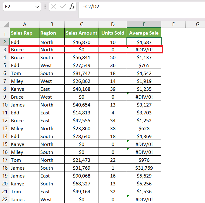
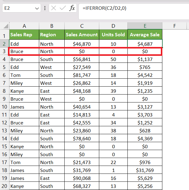
In this example, we have to calculate the average sale of each record by dividing the total sales amount by the units sold. However, when Excel attempts to divide 0 by 0, an error will be returned.
So, we need to handle division by zero errors gracefully.
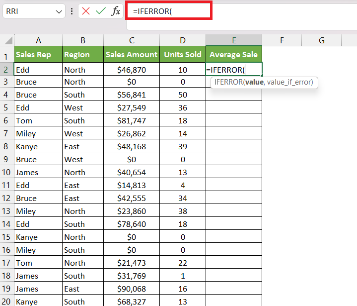
STEP 1: Enter the IFERROR function in a blank cell.
=IFERROR(
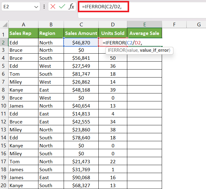
STEP 2: Enter the first argument – value. Here, we need to enter the formula first to calculate the average sale.
=IFERROR(C2/D2,
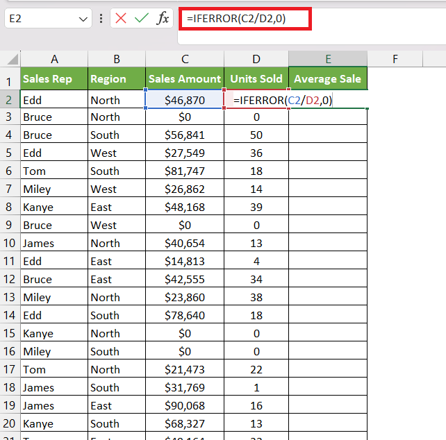
STEP 3: Enter the second argument – value_if_error. Here, we want “0” to be displayed if there is an error.
=IFERROR(C2/D2,0)
Apply the same formula to the rest of the cells by dragging the lower right corner downwards.
You now have all of the results!
Example 2 – Missing Data
IFERROR can be used to tell the user when the value you are searching for is missing in the dataset. Instead of showing an error, the function can show a message like this – “Not found”.
Let us look at an example of this.
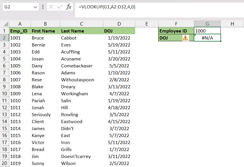
STEP 1: Here, we are using the VLOOKUP function to retrieve the Date of Joining of the employee ID mentioned in cell G1 by searching the dataset.
=VLOOKUP(G1,A2:D32,4,0)
- G1 represents the value we want to look up (Employee ID 1000).
- A2:D32 highlights the entire source data table.
- 4 indicates that we want to retrieve the date of joining, which is located in the fourth column.
- 0 ensures an exact match.
You will notice that there is a #N/A error value! This occurs because 1000 is not included in the source table. Let us make it look better with IFERROR!
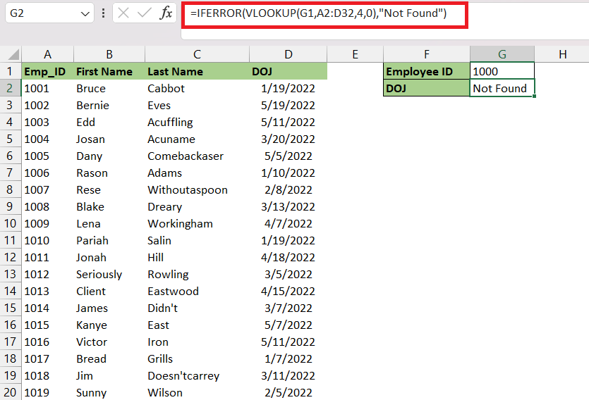
STEP 2: By wrapping the VLOOKUP formula with IFERROR, we can replace this error with a specified text, such as “Not Found”:
=IFERROR(VLOOKUP(G1,A2:D32,4,0), “Not Found”)
And just like that, your result is now clean and error-free!
The IFERROR function in Excel provides a powerful mechanism to handle errors and enhance user experience. It is versatile and an essential tool for anyone working with data and formulas in Excel.
Click here for the Top 20 Common Excel errors that you might face, or are currently facing and how to tackle them.
John Michaloudis is a former accountant and finance analyst at General Electric, a Microsoft MVP since 2020, an Amazon #1 bestselling author of 4 Microsoft Excel books and teacher of Microsoft Excel & Office over at his flagship MyExcelOnline Academy Online Course.

