Include Sparkline with Pivot Table

Once you have your Pivot Table ready and setup, you want to add something more graphical beside your data points. We have just the thing for you, you can include sparkline with pivot tables!

Key Takeaways

• Add Visual Trends Easily – You can insert Sparklines alongside Pivot Tables to provide mini charts that visually represent data trends without taking much space.

• Supports Multiple Sparkline Types – Excel allows you to use Line, Column, or Win/Loss Sparklines, giving flexibility based on the type of data in your Pivot Table.

• Dynamic Updates with Pivot Refresh – Sparklines automatically update when you refresh or filter the Pivot Table, ensuring your visuals always match the latest data.

• Ideal for Row-Based Analysis – Place Sparklines in a column next to the Pivot Table rows to quickly compare trends across categories, products, or regions.

• Format Sparklines for Better Insights – You can customize Sparkline styles, colors, and markers (like high and low points) to make key data trends stand out clearly.

Our Pivot Table Setup

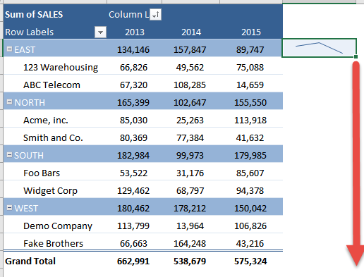
Here we have our Pivot Table ready:

See how you can do this in just a couple of steps.

How to Include Sparkline with Pivot Table

STEP 1: Select a spot right beside your Pivot Table. Go to Insert > Sparklines > Line

We want to create a sparkline based on our first row of data. Select the sales values of 2013-2015. Then click OK.

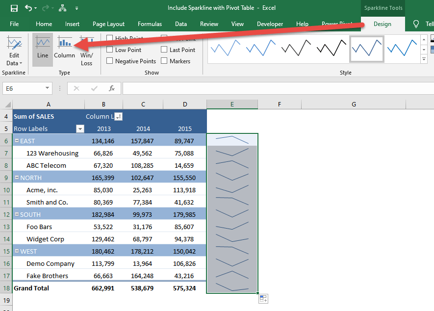
STEP 2: On the lower right corner, drag it all the way down to populate the rest of your table with sparklines.

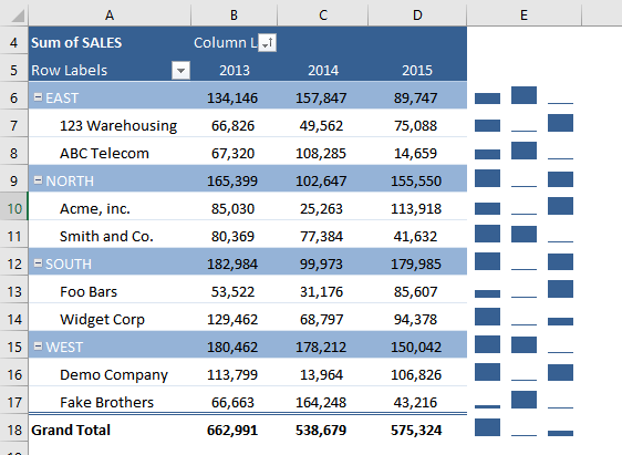
STEP 3: We can change the type as well. Go to Sparklines Tools > Design >Type > Column

You now have sparklines for your Pivot Table!

Frequently Asked Questions

What are Sparklines in Excel?
Sparklines are small, cell-sized charts that display trends or patterns in a row of data, like mini graphs embedded within a cell.

Can I insert Sparklines directly into a Pivot Table?
No, Sparklines can’t be placed inside the Pivot Table itself, but you can insert them in adjacent columns next to the Pivot Table rows.

Do Sparklines update when the Pivot Table data changes?
Yes, Sparklines are linked to the data range and will automatically refresh when you update, filter, or refresh the Pivot Table.

What types of Sparklines can I use with Pivot Tables?
Excel offers Line, Column, and Win/Loss Sparklines, all of which can be used alongside Pivot Table data based on your preferred visual style.

How do I format Sparklines for better visibility?
After inserting Sparklines, use the Sparkline Tools → Design tab to change colors, highlight high/low points, or adjust line styles for clear, meaningful visuals.

Bryan

Bryan Hong is an IT Software Developer for more than 10 years and has the following certifications: Microsoft Certified Professional Developer (MCPD): Web Developer, Microsoft Certified Technology Specialist (MCTS): Windows Applications, Microsoft Certified Systems Engineer (MCSE) and Microsoft Certified Systems Administrator (MCSA).

He is also an Amazon #1 bestselling author of 4 Microsoft Excel books and a teacher of Microsoft Excel & Office at the MyExecelOnline Academy Online Course.