The Ultimate Guide to Excel INDEX Function

When working with Excel, there are times when you need to pull specific information from a table or a range of data. The INDEX function is one of those powerful tools that can help me do just that. It allows me to retrieve a value from a specific location within a range, based on a given row and column number. If you’ve ever wondered how to pinpoint the exact cell in a dataset without scrolling through endless rows and columns, the INDEX function is the answer.

In this article, I’ll walk you through everything you need to know about using the Excel INDEX function, complete with real-world examples to ensure you can apply it in your own spreadsheets.

Key Takeaways:

• The INDEX function retrieves a value from a specific row and column in a range.
• INDEX offers more flexibility than VLOOKUP or HLOOKUP by allowing searches across any column or row.
• Combining INDEX with MATCH enhances dynamic lookups in large datasets.
• INDEX can handle dynamic ranges, making it adaptable to growing datasets.
• Error-handling and accurate range referencing are crucial for preventing common INDEX function errors.

 

Unlocking the Power of Excel’s INDEX Function

What is the Excel INDEX Function?

At its core, the INDEX function returns the value of a cell in a table based on its row and column numbers. Unlike other lookup functions, such as VLOOKUP or HLOOKUP, the INDEX function gives me much more flexibility when dealing with data spread across both rows and columns.

The syntax for the INDEX function is:

=INDEX(array, row_num, [column_num])

• array: This is the range of cells or array from which I want to retrieve data.
• row_num: This is the row number in the array.
• column_num: (Optional) This is the column number in the array.

 

Why INDEX is a Must-Know for Excel Users

As someone who frequents Excel, I can’t overstate the importance of the INDEX function. It’s a game-changer, especially for those who regularly delve into data analysis, reporting, or any task that involves handling large spreadsheets. INDEX saves significant time by pinpointing data without manual search, offering a direct route to the values you need.

It’s also a linchpin for collaborative work, enabling multiple users to access and edit specific information efficiently without stumbling over each other’s data points. Mastery of INDEX equips you with the agility to make swift adjustments and decisions—a must for dynamic business environments.

 

Example of Excel Index Function

Example 1: Using INDEX to Retrieve a Value from a Single Column

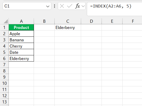
Let’s say I have a list of products in column A, and I want to know which product is in the fifth row. To retrieve the value from the fifth row, I can use the INDEX function like this:

=INDEX(A2:A6, 5)

When I hit enter, it returns “Elderberry.” The function simply pulls the value from the fifth row of the range I specified. It’s that straightforward!

Example 2: Using INDEX with a 2-Dimensional Array

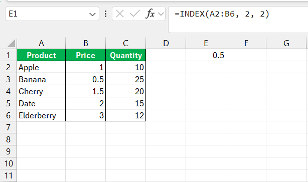
Now, let’s complicate things a bit. Imagine I have a table of products, their prices, and the quantities sold. My goal is to find the price of the second product on the list. In this case, if I want to retrieve the price of “Banana” (the second product), I can use the following formula:

=INDEX(A2:B6, 2, 2)

Here’s how it works:

• A2:B6: This is my array. It includes the “Product” and “Price” columns.
• 2: This is the row number. Since Banana is the second product, I input 2.
• 2: This is the column number. I want the price, which is in the second column.

After running this formula, Excel returns 0.50, which is the price of a Banana.

Example 3: Combining INDEX with MATCH for More Flexibility

While the INDEX function is powerful on its own, its true potential comes out when I combine it with the MATCH function. MATCH helps me find the position of a value in a range, and I can then use that position within the INDEX function to retrieve data.

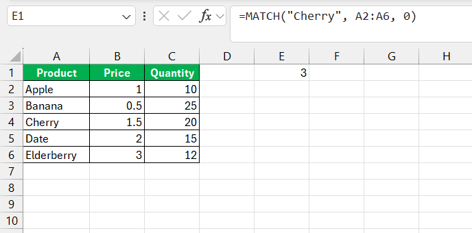
Let’s take a scenario where I want to find the quantity sold for a product without knowing its exact row number. Suppose I want to know the quantity sold for “Cherry.” To find the row where “Cherry” is listed, I use the MATCH function:

=MATCH(“Cherry”, A2:A6, 0)

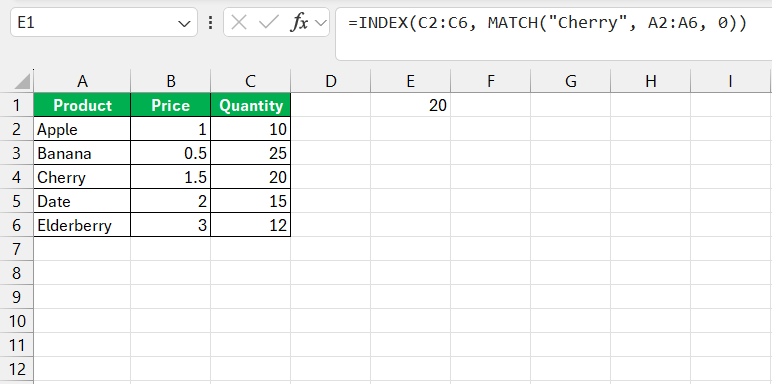
This formula returns 3 because “Cherry” is the third product in column A. Now, I can use this result inside my INDEX function to find the quantity sold:

=INDEX(C2:C6, MATCH(“Cherry”, A2:A6, 0))

This formula will give me the value from column C (the Quantity column), where “Cherry” is found in column A. The result is 20.

Example 4: Using INDEX with Dynamic Ranges

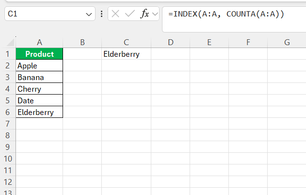
One of the best parts about the INDEX function is that I can make my ranges dynamic. For example, let’s say I want to return the last value in a column, but my dataset keeps growing over time. Rather than manually updating my range, I can create a dynamic range using the INDEX function.

To find the last value in column A, I can use this formula:

=INDEX(A:A, COUNTA(A:A))

Here, COUNTA counts the number of non-empty cells in column A. INDEX then returns the value in the row corresponding to that count. This way, even if I add more products to my list, this formula will always return the last product.

Common Pitfalls and How to Avoid Them

Navigating Through Common Errors

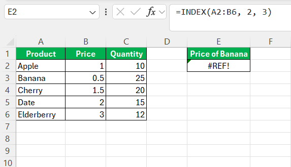
Even seasoned Excel users can stumble upon errors with the INDEX function, but learning to navigate them is part of the journey. ‘REF!’ errors crop up when the specified row or column is out of the defined range—a reminder to double-check boundaries.

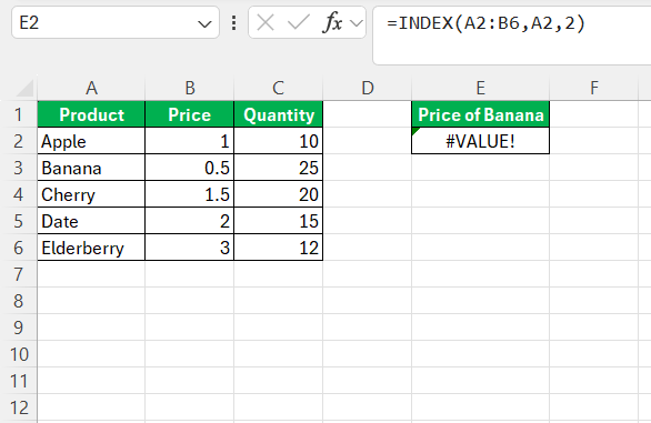
‘VALUE!’ errors typically signal that your row or column indicators aren’t numeric, prodding you to verify your inputs are correct.

These common mishaps can usually be remedied by a keen review of your function arguments and ensuring they align with the structure of your dataset. I always recommend troubleshooting one step at a time to pinpoint exactly where the discrepancy lies.

Tips for Ensuring Accurate Results

To ensure the INDEX function yields accurate results every time, follow these best practices: Firstly, confirm that your range references are spot on; mismatches here lead to incorrect outputs. Using named ranges can be helpful, as it reduces the chances of selecting incorrect cells. Secondly, remain vigilant when dragging your formula across cells; relative references can shift and alter the intended outcome.

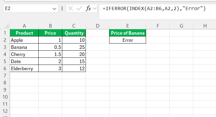
Thirdly, incorporate error-checking functions like IFERROR to neatly handle potential errors.

This preemptive measure keeps your spreadsheet professional and user-friendly. Complement these practices with regular data validation checks, and you’ll maintain the integrity of your results.

 

FAQ: Mastering Excel INDEX Function

What Are the Most Common Uses of the INDEX Function?

The INDEX function is commonly used to retrieve individual values from within a range, build dynamic named ranges, create advanced lookup formulas by pairing it with the MATCH function, and ensure formulas remain flexible and accurate as data changes. It’s also instrumental in creating interactive dashboards and complex financial models.

Can the INDEX Function Return Multiple Values?

Yes, INDEX can return multiple values if combined with other functions like SMALL or LARGE in an array formula setup. This allows you to retrieve a set of values that meet certain criteria from a larger dataset.

How Does INDEX Differ from Excel VLOOKUP and HLOOKUP?

INDEX differs from VLOOKUP and HLOOKUP primarily in its flexibility. Unlike VLOOKUP, which is limited to searching for values in the first column to the right, INDEX can retrieve from any column or row in a range. HLOOKUP searches horizontally across the top row, while INDEX doesn’t restrict the search direction and doesn’t require the data to be sorted.

Is It Possible to Use INDEX with Tables and Structured References?

Absolutely, INDEX can be used with tables and structured references in Microsoft Excel. This enhances readability and maintenance of your workbook because structured references are more intuitive than traditional cell references. They adapt automatically as your data in a table grows or shrinks, making INDEX even more powerful.

What Are the Best Practices When Using INDEX in Complex Formulas?

When integrating INDEX in complex formulas, best practices include using named ranges for clarity, pairing it with MATCH for dynamic lookups, and testing formulas on sample data before full-scale application. Always encapsulate with error-handling functions like IFERROR, and document your formulas for ease of understanding by others.